44 - Overfitting and regularization: L2, L1 and the high-accuracy trap

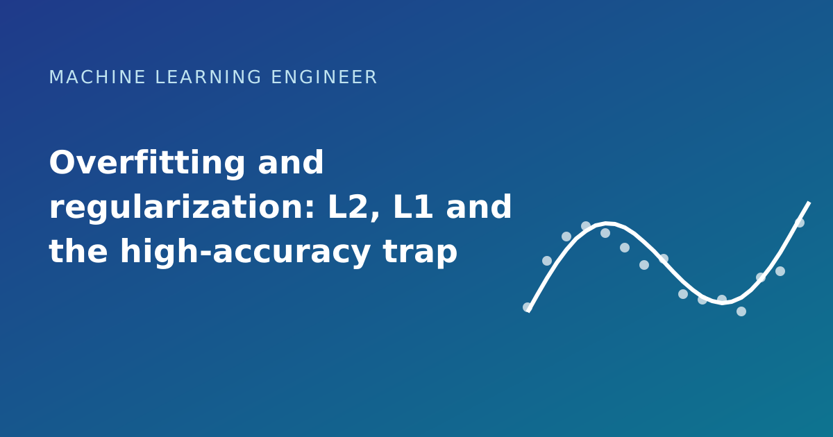
Two students prepare for an exam. The first memorizes the answers to the old exercises, commas included. The second understands the principles. On the old exercises the first gets top marks, the second a bit less; at the exam, with new questions, the second does much better. The first has overfit: it has adapted its knowledge to the noise and random details of the data it saw, and not to what holds in general. A model can do the same. Its error on the training data falls towards zero, and it looks like a victory; but on the real exam (never-seen data) it gets worse.

This lesson closes the block on regression with the main cure for overfitting: regularization, that is limiting the model's freedom by penalizing its complexity. You will see how it is derived, how it is implemented by hand, how L2 and L1 differ, and the accuracy trap that looks excellent and is not.

The words to pin down

The term that matters most is generalization: the ability of a model to work on new data. It is the only real goal, and the error on the training data is only a means of getting there. How far a model can adapt is called capacity (or complexity): a degree-15 polynomial has an enormous capacity, a line a low one. If the capacity is too small the model is wrong on both training and test (underfitting, high bias); if it is too large it does very well on training and badly on test (overfitting, high variance). Regularization is the set of techniques that reduce overfitting by limiting complexity; here it is a term added to the cost function that penalizes large weights. Its strength, λ, is a hyperparameter: a value chosen by you before training, selected with validation and never by looking at the test set.

The idea: a cost that punishes large weights

In the lesson on polynomial regression you saw that a degree-15 polynomial reaches a training error of 0.020 and a test error of 3.42, a hundred and seventy times worse. Its coefficients were of the order of billions: to make the curve pass close to every point, the model uses gigantic weights that compensate each other. A large weight means a small change in the input moves the output a lot: a "nervous" function, chasing noise. The idea is: if the cost also includes the size of the weights, the model will prefer, at equal error on the data, a solution with small weights, therefore smoother. In L2 regularization (or ridge) the sum of the squares of the weights is added:

J_L2(θ) = (1 / 2m) · Σ_i ( h(x_i) − y_i )²  +  (λ / 2m) · Σ_{j=1..n} θ_j²

The first term is the usual error. The second is the penalty, and λ ≥ 0 is the regularization strength: with λ = 0 there is no penalty (back to the original model); with very large λ the weights are crushed towards zero and the model becomes almost a constant. Note that the sum starts at j = 1: the intercept θ₀ is not penalized, because it does not measure the sensitivity to any feature, only the average level of the target. Penalizing it would make the solution depend on a constant added to the target: shifting all the y values by 100 would change the weights of the features, which have nothing to do with it.

What changes in the gradient and in the closed-form solution

Differentiating the penalty is easy: the derivative of (λ/2m)θ_j² with respect to θ_j is (λ/m)θ_j. The gradient becomes:

∂J/∂θ_j = (1/m) Σ_i (h(x_i) − y_i) x_ij  +  (λ/m) θ_j         (for j ≥ 1; for j = 0 the second term is missing)

In the update θ_j ← θ_j − α·∂J/∂θ_j the extra term means that at each step the weight is first "shrunk" by a factor (1 − αλ/m) and then corrected by the error gradient. This is why L2 is also called weight decay: in a neural network you will find it under this name. Careful, though: the equivalence between the L2 penalty and weight decay holds for plain gradient descent; for adaptive optimizers such as Adam the two do not coincide, which is why a "decoupled weight decay" variant exists (Loshchilov and Hutter, in the sources). The closed-form solution is obtained by setting the gradient to zero, as for linear regression:

θ = ( XᵀX + λ·D )⁻¹ Xᵀ y          with D = identity matrix, except D₀₀ = 0 (the intercept is not penalized)

A precious side effect: adding λ on the diagonal makes XᵀX + λD always invertible and well conditioned, even when the features are collinear or more numerous than the examples. Ridge therefore also cures the coefficient instability of the previous lesson.

Ridge by hand: the degree-15 polynomial tamed

We restart from the same data as the lesson on polynomial regression (noisy sine wave, 30 training points and 30 test points) and implement the closed-form solution with the penalty:

import numpy as np
from sklearn.model_selection import train_test_split
from sklearn.linear_model import Ridge

r = np.random.default_rng(1)
x = r.uniform(0, 6, 60)
y = np.sin(x) + r.normal(0, 0.25, 60)
x_tr, x_te, y_tr, y_te = train_test_split(x, y, test_size=0.5, random_state=1)

def powers(x, degree):
    return np.column_stack([x ** k for k in range(1, degree + 1)])

P_tr = powers(x_tr, 15)
mu, sd = P_tr.mean(axis=0), P_tr.std(axis=0)                              # standardization from the training set
A = np.column_stack([np.ones(30), (P_tr - mu) / sd])                      # (30, 16)
B = np.column_stack([np.ones(30), (powers(x_te, 15) - mu) / sd])          # (30, 16)

def ridge(A, y, lam):
    D = np.eye(A.shape[1]) * lam
    D[0, 0] = 0.0                                                         # the intercept is not penalized
    return np.linalg.solve(A.T @ A + D, A.T @ y)

print("lambda        train MSE   test MSE   max |theta|")
for lam in (0, 1e-4, 1e-2, 1e-1, 1, 10, 100):
    theta = ridge(A, y_tr, lam) if lam > 0 else np.linalg.lstsq(A, y_tr, rcond=None)[0]
    print("%-12g  %9.4f  %9.4f  %12.2f" % (lam, ((A @ theta - y_tr) ** 2).mean(), ((B @ theta - y_te) ** 2).mean(), np.abs(theta[1:]).max()))

sk = Ridge(alpha=1.0).fit(A[:, 1:], y_tr)
print("\ncomparison at lambda = 1: first coefficients by hand %s  sklearn %s" % (np.round(ridge(A, y_tr, 1.0)[:3], 5), np.round(np.r_[sk.intercept_, sk.coef_[:2]], 5)))

lambda        train MSE   test MSE   max |theta|
0                0.0196     3.4167  3403853961.78
0.0001           0.0259     0.0386         10.96
0.01             0.0328     0.0418          3.40
0.1              0.0488     0.0670          1.46
1                0.0920     0.1292          0.46
10               0.1246     0.1621          0.21
100              0.2562     0.3198          0.08

comparison at lambda = 1: first coefficients by hand [ 0.05268  0.01684 -0.45667]  sklearn [ 0.05268  0.01684 -0.45667]

What the code does. powers builds the columns x, x², ..., x¹⁵; they are standardized (without this step the weights of different powers would have incomparable scales and the penalty would hit arbitrarily, a point we return to among the traps). ridge is the closed formula; D[0, 0] = 0 leaves the intercept free. The loop scans seven values of λ and prints training error, test error and the largest coefficient in absolute value. Four readings:

• With λ = 0 (no regularization) the disaster is back: test 3.42 and coefficients of the order of billions.
• Already with λ = 10⁻⁴ the test collapses to 0.039 and the largest coefficient drops to 11: a tiny penalty is enough to heal the model. Training and test errors come closer.
• Beyond the optimal value the two errors rise together: with λ = 100 the model is too rigid (test 0.32, training 0.26). This is underfitting from excessive regularization.
• The training error always grows with λ (from 0.020 to 0.256): regularization sacrifices some fit to the data seen to gain generalization. The test error has a "U" shape (the picture above): λ is a compromise, and it is chosen by looking at validation.

Taken together, the four readings describe a curve and not a value to memorize: the penalty moves the model along the axis that goes from overfitting (zero λ, test 3.42) to underfitting (λ = 100, test 0.32 but with a training error of 0.26, higher than at any other point of the grid). The useful point lies in the middle, and in our numbers the minimum test error (0.039) falls at λ = 10⁻⁴, the smallest value of the grid after zero: it means that here a tiny penalty is enough, but also that the grid is not fine enough to say where the exact optimum is. The test set used as a guide in this example serves only to show the shape; in real work the same comparison is made on a validation set.

The final line confirms that the closed formula coincides with sklearn.linear_model.Ridge (where the alpha parameter is our λ, in the convention where the penalty is added to the sum of squared errors, not to the mean): identical first coefficients.

L1 (lasso): the regularization that switches features off

L1 regularization (lasso) penalizes the sum of the absolute values of the weights instead of their squares:

J_L1(θ) = (1 / 2m) · Σ_i ( h(x_i) − y_i )²  +  (λ / m) · Σ_j |θ_j|

The difference looks small but has a qualitative effect: L1 drives many weights exactly to zero, i.e. it selects features. The geometric intuition: with L2 the equivalent constraint "‖θ‖₂ ≤ c" is a circle (a sphere), smooth, and the solution touches the boundary at a generic point, with all components non-zero. With L1 the constraint "‖θ‖₁ ≤ c" is a diamond with its corners on the axes, and the level curves of the error tend to touch it precisely at the corners, where some components are zero.

Another, algebraic reading: the derivative of |θ| is ±1 even for tiny θ, so L1 pushes towards zero with constant force until the weight is cancelled; the derivative of θ² is 2θ, which vanishes as θ approaches zero, so L2 shrinks without ever zeroing. The absolute value is not differentiable at zero: subgradients or dedicated algorithms are used (coordinate descent in scikit-learn).

Let us compare the three approaches on a problem designed on purpose: 20 features, but only the first 5 really matter (true coefficients 3, −2, 1.5, 1, −1), the other 15 are noise, and only 50 examples to train on.

from sklearn.linear_model import LinearRegression, Lasso

rng = np.random.default_rng(0)
n, p = 100, 20
X = rng.normal(size=(n, p))
beta = np.zeros(p); beta[:5] = [3, -2, 1.5, 1, -1]                        # only 5 features matter
yy = X @ beta + rng.normal(0, 1, n)
Xs, Xt, ys, yt = train_test_split(X, yy, test_size=0.5, random_state=0)

print("model                test MSE   coefficients exactly 0 (out of 15 noise)   largest |coef| among the 15 noise ones")
for name, m in (("least squares", LinearRegression()), ("ridge  (alpha=1)", Ridge(alpha=1)),
                ("lasso  (alpha=0.05)", Lasso(alpha=0.05)), ("lasso  (alpha=0.1)", Lasso(alpha=0.1)), ("lasso  (alpha=0.5)", Lasso(alpha=0.5))):
    m.fit(Xs, ys)
    c = m.coef_
    print("%-20s %7.3f   %26d                       %10.3f" % (name, ((m.predict(Xt) - yt) ** 2).mean(), (np.abs(c[5:]) < 1e-8).sum(), np.abs(c[5:]).max()))
print("true coefficients of the first 5:  ", beta[:5])
print("lasso (alpha=0.1), first 5:        ", np.round(Lasso(alpha=0.1).fit(Xs, ys).coef_[:5], 2))

model                test MSE   coefficients exactly 0 (out of 15 noise)   largest |coef| among the 15 noise ones
least squares          1.705                            0                            0.391
ridge  (alpha=1)       1.772                            0                            0.408
lasso  (alpha=0.05)    1.416                            5                            0.230
lasso  (alpha=0.1)     1.367                            8                            0.204
lasso  (alpha=0.5)     2.875                           14                            0.013
true coefficients of the first 5:   [ 3.  -2.   1.5  1.  -1. ]
lasso (alpha=0.1), first 5:         [ 2.81 -1.8   1.13  1.1  -0.82]

What the code does. It generates a sparse problem (few truly relevant features), splits half and half between training and test and compares five models. Lasso with alpha = 0.1 zeroes 8 of the 15 noise features and obtains the best test (1.37 versus 1.71 for least squares). Increasing alpha zeroes more coefficients (14 out of 15 with alpha = 0.5), but the penalty also shrinks the true coefficients and introduces a systematic error (bias): the test error rises again to 2.88. Ridge with alpha = 1 does not improve on least squares (1.77 versus 1.71): it shrinks all coefficients, true ones included, and zeroes nothing. It is an honest result that contradicts the idea that "regularization always improves": it depends on the problem. With few true coefficients and a lot of noise, L1 helps more; with many features that each contribute a little, L2 is usually preferable.

Regularization in classification: C = 1/λ

Logistic regression is regularized in the same way, adding the penalty to the log-loss. In scikit-learn the parameter is C, the inverse of the strength: small C = strong regularization, huge C = none. Here the typical situation is "many features, few examples": 300 examples, 100 features of which only 5 are informative, training on 150.

from sklearn.datasets import make_classification
from sklearn.pipeline import make_pipeline
from sklearn.preprocessing import StandardScaler
from sklearn.linear_model import LogisticRegression
from sklearn.model_selection import GridSearchCV

Xc, yc = make_classification(n_samples=300, n_features=100, n_informative=5, n_redundant=0, class_sep=1.2, random_state=0)
Xa, Xb, ya, yb = train_test_split(Xc, yc, test_size=0.5, stratify=yc, random_state=0)

print("C           train accuracy   test accuracy   max |weight|")
for C in (1e4, 1, 0.1, 0.01, 0.001):
    m = make_pipeline(StandardScaler(), LogisticRegression(C=C, max_iter=5000)).fit(Xa, ya)
    print("%-10g  %14.3f   %13.3f   %12.2f" % (C, m.score(Xa, ya), m.score(Xb, yb), np.abs(m[-1].coef_).max()))

grid = GridSearchCV(make_pipeline(StandardScaler(), LogisticRegression(max_iter=5000)),
                    {"logisticregression__C": np.logspace(-4, 2, 13)}, cv=5).fit(Xa, ya)
print("\nC chosen with 5-fold CV on the training set only: %g   CV accuracy %.3f   test accuracy %.3f" % (
    grid.best_params_["logisticregression__C"], grid.best_score_, grid.score(Xb, yb)))

l1 = make_pipeline(StandardScaler(), LogisticRegression(l1_ratio=1, solver="liblinear", C=0.1)).fit(Xa, ya)
print("L1 with C=0.1: features with non-zero weight = %d out of 100, test accuracy %.3f" % ((l1[-1].coef_ != 0).sum(), l1.score(Xb, yb)))

C           train accuracy   test accuracy   max |weight|
10000                1.000           0.733           7.48
1                    1.000           0.760           2.23
0.1                  0.987           0.747           0.97
0.01                 0.947           0.767           0.29
0.001                0.927           0.733           0.05

C chosen with 5-fold CV on the training set only: 0.001   CV accuracy 0.773   test accuracy 0.733
L1 with C=0.1: features with non-zero weight = 6 out of 100, test accuracy 0.880

What the code does. The Pipeline puts the StandardScaler before the classifier (the penalty depends on feature scale, so standardizing is mandatory). In the first loop, with huge C (no regularization) the model reaches training accuracy 1.000 and test 0.733: overfitting in its classic form. Reducing C the training drops (0.927 with C = 0.001) and the test rises slightly (0.767 with C = 0.01): the gain is modest, because with 100 features and 150 examples the problem is hard for any L2 model. The second block shows the correct use: GridSearchCV chooses C with cross-validation on the training set only (here C = 0.001) and only afterwards the test is looked at. The result is instructive: cross-validation picks the strongest regularization on the grid (C = 0.001) and the test gives 0.733, equal to the unregularized model.

With 150 test examples, a single example is worth 0.0067, so the differences between 0.733 and 0.767 are 5 examples: sampling noise. There is no demonstrable gain from the L2 penalty alone on this problem. The last line is the surprise: the L1 penalty with C = 0.1 keeps only 6 features out of 100 active, almost exactly the 5 informative ones, and brings the test to 0.880. When the truth is sparse, selecting features matters more than shrinking them all. A version note: with scikit-learn 1.8.0 the penalty parameter is deprecated (in the signature its value is 'deprecated') and the penalty is chosen with l1_ratio: 0 is L2, 1 is L1. With earlier versions you write penalty="l1"; the liblinear solver supports L1.

The high-accuracy trap

In this lesson a reassuring accuracy number hid a problem in three different ways. The first is the comparison between training (1.000) and test (0.733): the number on the training set has no informative value, because a sufficiently flexible model always reaches it. The second is using the test set to choose λ or C: if you try ten values and keep the best on the test, that test has become a second training set and the score is optimistic; this is why there is GridSearchCV on the training set and the test stays intact for the final evaluation. The third concerns imbalanced classes, covered in the lesson on the process of an ML project: overfitting on a few positives changes overall accuracy little, since it is dominated by the negatives, so always compare precision and recall between training and validation.

Other ways to fight overfitting

• More data: the most effective cure, when available. For the same model, more examples make it harder to memorize noise.
• Simpler models: fewer features, lower degree, shallower trees.
• Early stopping: interrupt gradient descent when the validation error stops falling. It is an implicit form of regularization: small weights at the beginning and growing over time.
• Data augmentation, dropout: techniques specific to neural networks (you will see them later in the module).

The four items are not equivalent alternatives. The first two act on the problem (data and model), the others on the training procedure; the explicit regularization of this lesson sits in the middle and is the cheapest to try, because it is one line of code and one hyperparameter. When in doubt, start from the data, which no penalty replaces.

Trade-offs and traps

• L2 versus L1: L2 stabilizes and handles correlated features well (it shares the weight among them); L1 selects and produces compact models but, with correlated features, picks one almost at random and may change its choice as the data change. The combination is called elastic net.
• Forgetting standardization: the penalty applied to raw features hits more the features with small values (which require large weights) and less those with large values: an arbitrary effect due to the units of measure.
• Penalizing the intercept (avoided here).
• Choosing λ on the test set, or on the training set: always cross-validation.
• Mixing up alpha, λ and C: in scikit-learn Ridge(alpha) and Lasso(alpha) use different scale conventions from each other, and C is the inverse of λ. Check the documentation of the object you use.
• Leakage in validation: the scaler goes inside the Pipeline passed to GridSearchCV, otherwise the validation folds have already influenced the standardization.

The six items reduce to two families. The first is the choice of penalty (L1, L2, elastic net) and has an answer that depends on the problem, as the experiments in this lesson show. The second is the discipline of the procedure: standardize inside the pipeline, do not touch the intercept, choose the strength only with validation. The most costly errors almost always come from the second family, because they produce good and false scores without any warning.

Bias and variance measured: why a bit of distortion pays off

The reason regularization works can be measured with a simulation. We fix the truth (20 features, of which only 5 have non-zero coefficients: 3, 2, 1.5, 1, 0.5), generate 2,000 independent datasets of 40 examples with noise of deviation 2, and on each one train the model and predict the value at a same fixed point x. Since we know the true value at that point, we can decompose the mean squared error into bias² (how far the mean of the predictions, across datasets, is from the truth) and variance (how much the predictions fluctuate from one dataset to another). MSE = bias² + variance holds (plus the irreducible noise, which we do not count here because we compare with the noise-free value).

from sklearn.linear_model import Lasso, ElasticNet, lasso_path

rng_r = np.random.default_rng(0)
n_features, n_samples = 20, 40
true_beta = np.array([3, 2, 1.5, 1, 0.5] + [0] * 15, dtype=float)
x_query = rng_r.normal(size=(1, n_features))
true_value = float((x_query @ true_beta)[0])

alphas = (0, 1, 5, 20, 100)                                                 # 0 = least squares without penalty
predictions = {a: [] for a in alphas}
for repetition in range(2000):
    gen = np.random.default_rng(100 + repetition)
    X_sim = gen.normal(size=(n_samples, n_features))
    y_sim = X_sim @ true_beta + gen.normal(0, 2, n_samples)
    for a in alphas:
        model = LinearRegression() if a == 0 else Ridge(alpha=a)
        predictions[a].append(float(model.fit(X_sim, y_sim).predict(x_query)[0]))

print("true value at the point: %.3f" % true_value)
print("alpha (ridge)   bias²     variance   total MSE")
for a in alphas:
    v = np.array(predictions[a])
    print("%-14g   %.4f    %.4f     %.4f" % (a, (v.mean() - true_value) ** 2, v.var(), ((v - true_value) ** 2).mean()))

true value at the point: 0.911
alpha (ridge)   bias²     variance   total MSE
0                0.0016    3.5930     3.5946
1                0.0057    2.9343     2.9399
5                0.0315    1.9987     2.0302
20               0.1411    1.3215     1.4626
100              0.4419    0.6957     1.1376

What the code does. For each value of alpha it trains 2,000 models on different datasets and measures, at the fixed point (true value 0.911), the square of the gap between the mean prediction and the truth (bias²) and the variance of the predictions. Without penalty (alpha = 0) the bias² is almost null (0.0016), as expected from an unbiased estimator, but the variance is 3.593: with 40 examples and 20 features the predictions fluctuate a lot from one sample to the other. Increasing alpha the bias² grows (0.0057, 0.0315, 0.1411, 0.4419) and the variance falls much faster (2.934, 1.999, 1.322, 0.696).

The total MSE falls from 3.595 to 1.138: with alpha = 100 the error is about a third of that of least squares, paying a bias² of 0.44. This is the bias–variance trade-off in numerical form: a model slightly wrong on average (biased toward zero) but stable beats the model that is right on average but unstable. Two caveats. First, in this experiment the MSE has not yet stopped falling at alpha = 100, so the optimum is beyond the tested grid: exercise 1 proposes looking for it. Second, it is a single prediction point: the bias changes from point to point, and in practice alpha is chosen with cross-validation over many points, not with a simulation that requires knowing the truth.

The penalty depends on the scale of the features: standardize first

The ridge penalty sums the squares of the coefficients. But a coefficient depends on the unit of measure of the feature: if you express a length in millimetres instead of metres, its coefficient becomes a thousand times smaller, and is therefore penalized much less. The result is that regularization arbitrarily favours features with a large scale. We show it with two features of identical importance (true coefficient 1 for both), where we multiply the first by a factor s.

n_s = 300
f1, f2 = rng_r.normal(size=n_s), rng_r.normal(size=n_s)
target = f1 + f2 + rng_r.normal(0, 0.5, n_s)

print("scale s of the first feature   ridge coefficients (alpha=100)   effect in original units (coef × s)   after standardization")
for s in (1, 10, 100):
    X_scaled = np.column_stack([f1 * s, f2])
    raw = Ridge(alpha=100).fit(X_scaled, target).coef_
    standardized = Ridge(alpha=100).fit(StandardScaler().fit_transform(X_scaled), target).coef_
    print("%-28d   %-31s   %-37s   %s" % (s, np.round(raw, 3), np.round(raw * np.array([s, 1]), 3), np.round(standardized, 3)))

scale s of the first feature   ridge coefficients (alpha=100)   effect in original units (coef × s)   after standardization
1                              [0.781 0.767]                     [0.781 0.767]                           [0.793 0.758]
10                             [0.102 0.762]                     [1.023 0.762]                           [0.793 0.758]
100                            [0.01  0.762]                     [1.026 0.762]                           [0.793 0.758]

What the code does. Two features have the same true coefficient (1). With s = 1 ridge treats them similarly (0.781 and 0.767). Multiplying the first by 10 its coefficient falls to 0.102: it has a scale ten times larger, so to produce the same effect a coefficient ten times smaller is needed, and the penalty on the square punishes it much less. Converted to original units (coefficient × s) the effect of the first feature is 1.023, against 0.762 for the second: the feature with the larger scale has been shrunk less, only as a matter of unit of measure. With s = 100 the coefficient is 0.01 and the effect 1.026.

After standardization, instead, the two features are treated identically for every s (0.793 and 0.758, the values do not depend on s), and the result no longer depends on units. The rule is simple and non-negotiable: every model with a penalty on the coefficients (ridge, lasso, elastic net, logistic regression with C) requires standardized features, and the standardization must be computed only on the training set and inside the cross-validation pipeline (otherwise it leaks information, as seen in the first lesson of the module). A useful variant: do not penalize the intercept, which scikit-learn already does.

Correlated features: lasso chooses, elastic net splits, ridge distributes

When several features carry the same information, the three kinds of penalty behave differently. Lasso (L1) tends to choose some and weigh them arbitrarily and unstably (with a stronger penalty it zeroes others). Ridge (L2) distributes the weight among all. The elastic net combines the two penalties, α·(l1_ratio·Σ|w| + (1 − l1_ratio)/2·Σw²), and tends to keep together groups of correlated features while still zeroing the useless ones. We create four noisy copies of the same signal z (deviation 0.1) plus four features of pure noise, with target 4·z + noise.

z = rng_r.normal(size=200)
X_corr = np.column_stack([z + rng_r.normal(0, 0.1, 200) for _ in range(4)] + [rng_r.normal(size=200) for _ in range(4)])
y_corr = 4 * z + rng_r.normal(0, 1, 200)

print("coefficients of the 8 features: the first 4 are copies of the signal, the last 4 are noise")
for name, model in (("lasso (alpha=0.1)", Lasso(alpha=0.1)), ("elastic net (alpha=0.1, l1_ratio=0.5)", ElasticNet(alpha=0.1, l1_ratio=0.5)), ("ridge (alpha=10)", Ridge(alpha=10))):
    coefficients = model.fit(X_corr, y_corr).coef_
    print("%-38s %s     sum of the first 4: %.2f" % (name, np.round(coefficients, 2), coefficients[:4].sum()))

coefficients of the 8 features: the first 4 are copies of the signal, the last 4 are noise
lasso (alpha=0.1)                      [ 1.44  1.67  0.34  0.45 -0.   -0.02  0.   -0.  ]     sum of the first 4: 3.89
elastic net (alpha=0.1, l1_ratio=0.5)  [ 1.05  1.09  0.87  0.89 -0.03 -0.06  0.   -0.  ]     sum of the first 4: 3.90
ridge (alpha=10)                       [ 1.05  1.1   0.91  0.88 -0.09 -0.1   0.04 -0.03]     sum of the first 4: 3.94

What the code does. With four nearly identical copies of the signal and four noise features, the three models estimate very different coefficients on the first four, but with a nearly equal sum (3.89, 3.90, 3.94 vs the value 4 that the truth requires). Lasso with alpha = 0.1 weighs the four copies very unequally: [1.44, 1.67, 0.34, 0.45]. With another draw of the data the proportions would be different, because the model has no reason to prefer one copy over another: it is the instability cited as a defect of lasso with correlated features. In this experiment, with this alpha, it does not zero any; with higher alpha it would zero some.

The elastic net with l1_ratio = 0.5 keeps them together with much more similar weights ([1.05, 1.09, 0.87, 0.89]) and ridge splits them almost equally ([1.05, 1.10, 0.91, 0.88]). On the four pure-noise features, lasso and elastic net give almost or exactly zero coefficients (from −0.06 to 0.00), while ridge leaves small but non-zero ones (from −0.10 to 0.04): this is the fundamental difference, because ridge never selects, it only shrinks. Which to choose? If you think few features really matter and want a readable model, lasso; if many contribute a little each or the features are strongly correlated, ridge or elastic net; when in doubt, the elastic net with l1_ratio chosen by cross-validation is the most prudent starting point.

The lasso regularization path: features enter one at a time

X_path = rng_r.normal(size=(100, 10))
true_path = np.array([3, -2, 1, 0.5, 0, 0, 0, 0, 0, 0.])
y_path = X_path @ true_path + rng_r.normal(0, 1, 100)
alpha_grid, coefficients, _ = lasso_path(X_path, y_path, alphas=[2, 1, 0.5, 0.2, 0.1, 0.02])

print("alpha   non-zero features   coefficients of the first 4 (true: 3, −2, 1, 0.5)")
for a, column in zip(alpha_grid, coefficients.T):
    print("%-6g  %-18d   %s" % (a, np.count_nonzero(column), np.round(column[:4], 2)))

alpha   non-zero features   coefficients of the first 4 (true: 3, −2, 1, 0.5)
2       2                    [ 0.63 -0.51  0.    0.  ]
1       2                    [ 1.72 -1.17  0.    0.  ]
0.5     3                    [ 2.3  -1.53  0.23  0.  ]
0.2     4                    [ 2.69 -1.77  0.61  0.24]
0.1     4                    [ 2.83 -1.85  0.74  0.36]
0.02    8                    [ 2.93 -1.91  0.85  0.44]

What the code does. With 100 examples and 10 features, of which only 4 have a non-zero coefficient (3, −2, 1, 0.5), it computes the lasso for six decreasing values of alpha. With alpha = 2 only two features enter (the two strongest) with greatly reduced coefficients (0.63 and −0.51: lasso shrinks everything toward zero, even what it keeps). With alpha = 0.5 a third enters (0.23), with alpha = 0.2 a fourth (0.24) and the coefficients grow toward the true values: 2.69, −1.77, 0.61, 0.24. With alpha = 0.1 the four true features are still the only active ones (2.83, −1.85, 0.74, 0.36): this is the range in which lasso does what it promises, the correct selection.

With alpha = 0.02 they have become eight: four pure-noise features have also entered (with small coefficients), while the four true coefficients are now close to those of least squares (2.93, −1.91, 0.85, 0.44). Note also that the true coefficients are never recovered exactly (the true 3 is estimated 2.93 even with the minimum penalty): it is the noise of the sample, not of the regularization. The operating message is twofold. First: the choice of alpha is not a detail, it is the act of deciding how many features to keep, and it is done with cross-validation. Second: lasso selects well only in a range of alpha; outside that range it removes signal (high alpha) or lets noise in (low alpha).

Three exercises

Exercise 1. Extend the alpha grid of the bias–variance simulation to 1,000 and 10,000: where is the minimum of the total MSE at that point? What happens to bias²? Why is it not enough to look at a single point to choose alpha? Exercise 2. In the scale experiment, repeat with lasso instead of ridge: which feature is zeroed first when s = 100, and why? Exercise 3. In the lasso path use cross-validation (LassoCV) to choose alpha and compare the number of selected features with the true number (4): does lasso select more or fewer, and how is it explained?

What you can do now

You can write ridge by hand and recognize that it coincides with scikit-learn's, choose λ or C with cross-validation without touching the test set, and decide between L2, L1 and elastic net according to the structure of the problem. You can also measure the bias-variance trade-off with a simulation and you know why standardization, inside the pipeline, is not optional. With this lesson you have closed the round on linear models (the previous one is logistic regression); the next step is the neuron, the perceptron and the reason why non-linear activation functions are needed.

Other lessons in the series that link to this one: Constrained Optimisation: Lagrange Multipliers, Duality and the KKT Conditions, Bayesian Statistics: Priors, Posteriors, Conjugates and Why Regularisation Is a Belief, Multivariate and polynomial regression, and feature scaling.