19 - Random Variables and Distributions

Machine Learning Engineer course · Module 02 · Mathematics and statistics · Lesson 4

Goal. Turn the outcomes of an experiment into numbers, describe their behaviour with their distribution, and summarise it with two indicators: the expected value (where the centre is) and the variance (how much it spreads). At the end you know the distributions you will meet everywhere (Bernoulli, binomial, Poisson, uniform, exponential, normal), you can derive their mean and variance, and you have seen with simulations the law of large numbers and the central limit theorem, including the case in which they do not work.

Myth to dispel. "Everything in nature is distributed like a bell (normal)." Many phenomena (waiting times, file sizes, wealth) have long tails in which the normal is wrong by orders of magnitude, and for some distributions the mean does not exist. We will show it with an experiment.

Introduction

In the previous lesson probability was a function on events (sets). But data are numbers: the height of a person, the number of clicks, the waiting time. A random variable is the bridge: it assigns a number to every outcome. On these numbers you can do what you do with numbers (means, sums, comparisons), keeping the rigour of probability. The terms needed are explained here at first use and summarised in the final glossary.

The path goes from the definition of random variable to expected value and variance, then to the notable distributions (Bernoulli, binomial, Poisson, uniform, exponential, normal), to the law of large numbers and the central limit theorem, and ends with the case in which these theorems do not hold (heavy tails) and with covariance and correlation. You need the probability concepts and the binomial coefficients of the previous lessons.

Random variables

The analogy: the token with the number

Every outcome of the experiment receives a numerical label, like a token with a number printed on it. You roll two dice: the outcome is the pair (3, 5), but you are interested in the sum 8. The sum is a random variable X: a function from the sample space Ω to the real numbers, X : Ω → ℝ (lesson 1 on functions, now applied). "Random" because it depends on the outcome, which you do not know in advance.

Two families are distinguished:

• Discrete: takes a countable list of values (the score of a die, the number of clicks).
• Continuous: takes any value in an interval (a time, a length).

The distinction matters because it changes the tool: for discrete variables you sum masses, for continuous ones you integrate densities. Almost everything that follows has two versions, one with sums and one with integrals, and it is the same idea written twice; we will use sums for the proofs and simulations for the continuous case.

Discrete variables: the mass function. The probability mass function (PMF) p(x) = P(X = x) says how much probability "weighs" on each value. The masses are non-negative and sum to 1.

Continuous variables: the density. For a continuous variable the probability of a precise value is zero (nobody has a height of exactly 175.000000... cm). One speaks instead of a density function f(x): the probability of falling between a and b is the area under the curve between a and b. The analogy is the density of a material: a piece of metal has a density at every point, but the mass is a single number for finite volumes. So a density can exceed 1 (it is a height, not a probability); only its total area equals 1. (We make the concept of area under a curve precise in the calculus lesson.)

The distribution function (CDF) F(x) = P(X ≤ x) works for both: it is non-decreasing, starts from 0 and reaches 1.

from itertools import product
from fractions import Fraction
from collections import Counter

# exact PMF of the sum of two dice: count the pairs for each sum
conteggio = Counter(a + b for a, b in product(range(1, 7), repeat=2))
pmf = {x: Fraction(c, 36) for x, c in sorted(conteggio.items())}
print("PMF:", {x: str(p) for x, p in pmf.items()})
print("sum of the masses:", sum(pmf.values()))

cdf, acc = {}, Fraction(0)
for x, p in pmf.items():
    acc += p
    cdf[x] = acc
print("F(7) = P(X <= 7) =", cdf[7], "| F(12) =", cdf[12])

Output obtained:

PMF: {2: '1/36', 3: '1/18', 4: '1/12', 5: '1/9', 6: '5/36', 7: '1/6', 8: '5/36', 9: '1/9', 10: '1/12', 11: '1/18', 12: '1/36'}
sum of the masses: 1
F(7) = P(X <= 7) = 7/12 | F(12) = 1

What the code does. Counter counts, for each value of the sum, in how many of the 36 pairs it appears; dividing by 36 gives the PMF with exact fractions (lesson 3). The second part builds the CDF by accumulating the masses in order: F(7) = 21/36 = 7/12. We check that the masses sum to 1 (first axiom) and that F(12) = 1.

Expected value: the centre of mass

The analogy: the balance point

Place weights on the axis of numbers, each at x with mass p(x). The point at which the axis balances on the tip of a finger is the expected value E[X] (or μ, "mu"):

E[X] = Σₓ x · p(x) (for continuous variables: ∫ x f(x) dx).

It is a mean weighted with the probabilities. It is not necessarily a value that X can take: the die is worth 3.5 on average, but 3.5 never comes up.

The property that simplifies everything: linearity

E[aX + b] = a·E[X] + b and E[X + Y] = E[X] + E[Y], even when X and Y are not independent.

Proof of the sum (discrete case). With the joint distribution p(x, y): E[X + Y] = Σₓ Σᵧ (x + y) p(x, y) = Σₓ x Σᵧ p(x, y) + Σᵧ y Σₓ p(x, y). The inner sums are the marginal distributions: Σᵧ p(x, y) = p_X(x) and Σₓ p(x, y) = p_Y(y). Hence E[X + Y] = Σₓ x p_X(x) + Σᵧ y p_Y(y) = E[X] + E[Y]. ∎ No assumption of independence was needed.

This linearity allows an elegant calculation: the expected value of the sum of two dice is 3.5 + 3.5 = 7, without a table.

E_dado = sum(Fraction(x, 6) for x in range(1, 7))
E_somma_pmf = sum(x * p for x, p in pmf.items())
print("E[die]            =", E_dado, "=", float(E_dado))
print("E[sum] from PMF   =", E_somma_pmf)
print("E[sum] linearity  =", 2 * E_dado)

# Linearity holds even with dependence: number of fixed points of a random permutation
import numpy as np
rng = np.random.default_rng(5)
n = 10
punti_fissi = [(rng.permutation(n) == np.arange(n)).sum() for _ in range(100_000)]
print("simulated mean of the fixed points:", round(float(np.mean(punti_fissi)), 3), "| theory: 1")

Output obtained:

E[die]            = 7/2 = 3.5
E[sum] from PMF   = 7
E[sum] linearity  = 7
simulated mean of the fixed points: 1.002 | theory: 1

What the code does. The first part computes E in two ways (from the PMF and by linearity) and finds 7. The second is an example in which linearity shines: a random permutation of n elements has, on average, exactly one fixed point (an element left in its place), for any n. Proof: let Iᵢ be the indicator "element i stays in place i". P(Iᵢ = 1) = 1/n and E[Iᵢ] = 1/n. The fixed points are ΣIᵢ, and by linearity E[ΣIᵢ] = n · (1/n) = 1. The Iᵢ are dependent on each other, but it does not matter. The simulation confirms.

Variance: the dispersion

Two restaurants serve on average 100 covers an evening: one always serves between 98 and 102, the other between 20 and 180. They have the same expected value, but different lives. The variance measures how far a variable moves on average from its expected value, squared:

Var(X) = E[(X − μ)²].

Why the square? Positive and negative deviations would offset each other (the mean of the deviations is always zero, by the definition of μ); squaring makes them all positive and penalises large deviations more. The unit of measure however becomes the square of the original (metres²), so one uses the standard deviation σ = √Var(X), which returns to the unit of X.

The formula for calculation

Expanding the square and using linearity:

Var(X) = E[X² − 2μX + μ²] = E[X²] − 2μ·E[X] + μ² = E[X²] − 2μ² + μ² = E[X²] − μ².

In words: "mean of the squares minus square of the mean". Properties: Var(aX + b) = a²·Var(X) (shifting does not change the dispersion, scaling by a multiplies it by a²); if X and Y are independent, Var(X + Y) = Var(X) + Var(Y).

E2_dado = sum(Fraction(x * x, 6) for x in range(1, 7))
var_dado = E2_dado - E_dado ** 2
print("E[X^2] =", E2_dado, "| Var(die) = E[X^2] - E[X]^2 =", var_dado, "=", round(float(var_dado), 4))

var_somma = sum((x - E_somma_pmf) ** 2 * p for x, p in pmf.items())
print("Var(sum of 2 dice) =", var_somma, "| 2 * Var(die) =", 2 * var_dado, "(independence)")
print("standard deviation of the die:", round(float(var_dado) ** 0.5, 4))

Output obtained:

E[X^2] = 91/6 | Var(die) = E[X^2] - E[X]^2 = 35/12 = 2.9167
Var(sum of 2 dice) = 35/6 | 2 * Var(die) = 35/6 (independence)
standard deviation of the die: 1.7078

What the code does. It computes Var(die) = 91/6 − (7/2)² = 35/12 from the formula "mean of the squares minus square of the mean", then the variance of the sum of two dice directly from the definition, and shows that it coincides with 2·Var(die): two dice are independent, so the variances add (and not the standard deviations, which add "in quadrature").

The notable distributions

Bernoulli: the coin

A single experiment with two outcomes: success (1) with probability p, failure (0) with 1 − p. E[X] = p, Var(X) = p(1−p) (because X² = X, so E[X²] = p and Var = p − p²). It is the brick of everything.

Binomial: the count of successes

Repeat n independent Bernoulli trials: how many successes k do you get? Each sequence with k successes and n − k failures has probability pᵏ(1−p)ⁿ⁻ᵏ (independence: you multiply); the sequences of that type are as many as the ways of choosing which k trials succeed, that is C(n, k) (lesson 2). Hence

P(X = k) = C(n, k) · pᵏ · (1−p)ⁿ⁻ᵏ.

To obtain mean and variance there is no need to compute complicated sums: X is the sum of n independent Bernoullis, so by linearity E[X] = np and, by independence, Var(X) = np(1−p).

import math

def binomiale_pmf(k, n, p):
    return math.comb(n, k) * p ** k * (1 - p) ** (n - k)

n, p = 20, 0.3
pm = [binomiale_pmf(k, n, p) for k in range(n + 1)]
media = sum(k * q for k, q in enumerate(pm))
var = sum(k * k * q for k, q in enumerate(pm)) - media ** 2
print("sum of the masses:", round(sum(pm), 12))
print("mean from PMF:", round(media, 6), "| n*p =", n * p)
print("variance from PMF:", round(var, 6), "| n*p*(1-p) =", n * p * (1 - p))

rng = np.random.default_rng(7)
campione = rng.binomial(n, p, size=200_000)
print("simulation: mean", round(float(campione.mean()), 3), "| variance", round(float(campione.var()), 3))

Output obtained:

sum of the masses: 1.0
mean from PMF: 6.0 | n*p = 6.0
variance from PMF: 4.2 | n*p*(1-p) = 4.199999999999999
simulation: mean 6.003 | variance 4.17

What the code does. It implements the formula with math.comb, verifies its normalisation (sum 1) and computes mean and variance from the definition, finding np and np(1−p) again. The last line generates 200,000 binomials with NumPy: sample mean and variance are close to the theoretical values.

Poisson: rare events

How many clicks arrive in a minute, how many errors on a page? Imagine the minute divided into n instants, in each an event with probability p = λ/n (with λ the mean number per minute). The count is binomial; for large n and small p, with λ = np fixed, C(n,k)pᵏ ≈ nᵏ/k! · (λ/n)ᵏ = λᵏ/k! and (1−λ/n)ⁿ⁻ᵏ → e⁻λ (a notable limit that we will see in the calculus lesson). The result is the Poisson distribution:

P(X = k) = e^(−λ) · λᵏ / k!, with E[X] = Var(X) = λ.

lam = 3.0
n_grande, p_piccolo = 1000, lam / 1000
print(" k | binomial(1000, 0.003) | Poisson(3)")
for k in range(0, 8):
    b = binomiale_pmf(k, n_grande, p_piccolo)
    po = math.exp(-lam) * lam ** k / math.factorial(k)
    print(f"{k:>2} | {b:21.5f} | {po:10.5f}")

Output obtained:

 k | binomial(1000, 0.003) | Poisson(3)
 0 |               0.04956 |    0.04979
 1 |               0.14914 |    0.14936
 2 |               0.22415 |    0.22404
 3 |               0.22438 |    0.22404
 4 |               0.16828 |    0.16803
 5 |               0.10087 |    0.10082
 6 |               0.05033 |    0.05041
 7 |               0.02151 |    0.02160

What the code does. It compares the binomial PMF with n = 1000 and p = 0.003 and the Poisson PMF with λ = 3: they coincide at the third or fourth digit. The Poisson is the right approximation for counts of rare events in an interval; it has the characteristic that mean and variance are equal, a quick check to understand whether counts are really "Poissonian" (if the variance is much larger than the mean, there is overdispersion and something else is needed).

Uniform: no preference

Constant density on [a, b]: f(x) = 1/(b−a). E = (a+b)/2, Var = (b−a)²/12. It is the distribution of basic random number generators (rng.random()), from which all the others are built.

Exponential: the waiting time

If events arrive with intensity λ per unit of time, the time to the next one has density f(x) = λe^(−λx) for x ≥ 0, with E = 1/λ and Var = 1/λ². It has the memoryless property: P(X > s + t | X > s) = P(X > t). Having already waited s does not change how much remains to wait. Proof: P(X > x) = e^(−λx), so P(X > s+t | X > s) = P(X > s+t)/P(X > s) = e^(−λ(s+t))/e^(−λs) = e^(−λt). ∎

rng = np.random.default_rng(3)
tempi = rng.exponential(scale=1 / 0.5, size=400_000)        # λ = 0.5, theoretical mean 2
print("mean:", round(float(tempi.mean()), 3), "| theory 1/λ =", 2.0)
s, t = 1.5, 2.0
cond = (tempi[tempi > s] > s + t).mean()
print(f"P(X > {s + t} | X > {s}) simulated = {cond:.4f} | P(X > {t}) = {(tempi > t).mean():.4f} | theory e^(-λt) = {math.exp(-0.5 * t):.4f}")

Output obtained:

mean: 2.005 | theory 1/λ = 2.0
P(X > 3.5 | X > 1.5) simulated = 0.3677 | P(X > 2.0) = 0.3694 | theory e^(-λt) = 0.3679

What the code does. It generates exponential times with λ = 0.5 (mean 2). Then it computes the conditional probability of exceeding s + t given that s has been exceeded: filtering the times beyond s (the "narrowed room" of lesson 3) and counting how many exceed s + t. The value coincides with the unconditional probability of exceeding t: the exponential does not remember.

Normal: the bell

N(μ, σ²) has density

f(x) = (1 / (σ√(2π))) · exp(−(x − μ)² / (2σ²)).

It has a symmetric shape, centred at μ, as wide as σ. Any normal is brought back to the standard normal N(0, 1) with the standardisation Z = (X − μ)/σ (the same operation as in the NumPy lesson). A memorable property (68-95-99.7 rule): the probability of falling within kσ of the mean is erf(k/√2), with erf the error function.

for k in (1, 2, 3):
    print(f"P(|Z| <= {k}) = {math.erf(k / math.sqrt(2)):.4f}")
print("exact value 1.96:", round(math.erf(1.96 / math.sqrt(2)), 4), "(the 95 % used in confidence intervals)")

from scipy import stats
print("check with SciPy:", round(stats.norm.cdf(2) - stats.norm.cdf(-2), 4))

Output obtained:

P(|Z| <= 1) = 0.6827
P(|Z| <= 2) = 0.9545
P(|Z| <= 3) = 0.9973
exact value 1.96: 0.95 (the 95 % used in confidence intervals)
check with SciPy: 0.9545

What the code does. math.erf(k/√2) gives the probability within ±kσ: 0.6827, 0.9545, 0.9973. 1.96 is the value that leaves 2.5% in each tail (95% in the centre): you will find it again in the confidence intervals. The last line confirms it with scipy.stats.norm, the reference library for distributions.

Why it is so important. Not because "nature is normal", but because of the central limit theorem, which we see shortly.

Chebyshev and the law of large numbers

Markov and Chebyshev

Markov's inequality. If Y ≥ 0 and a > 0, then P(Y ≥ a) ≤ E[Y] / a. Proof: E[Y] = E[Y·1{Y<a}] + E[Y·1{Y≥a}] ≥ 0 + a·P(Y ≥ a), because on the event Y ≥ a the value of Y is at least a. Dividing by a gives the claim. ∎

Chebyshev's inequality. Applying Markov to Y = (X − μ)² with a = (kσ)²: P(|X − μ| ≥ kσ) = P((X−μ)² ≥ k²σ²) ≤ σ²/(k²σ²) = 1/k². In words: any distribution with finite variance has at most 1/k² probability beyond k standard deviations (at most 25% beyond 2σ, 11% beyond 3σ). It is a coarse bound but valid for all.

The law of large numbers

Let X̄ₙ be the mean of n independent observations with the same mean μ and variance σ². Then E[X̄ₙ] = μ and Var(X̄ₙ) = σ²/n (the variances add, then the factor 1/n² divides by n). By Chebyshev:

P(|X̄ₙ − μ| ≥ ε) ≤ σ² / (n ε²) → 0 for n → ∞.

The sample mean approaches the true mean, with a dispersion that falls as σ/√n: to halve the error you need four times the data.

rng = np.random.default_rng(11)
mu, sigma = 2.0, 2.0                                   # exponential with mean 2 and standard deviation 2
eps = 0.25
print("   n | simulated P(|mean - μ| >= 0.25) | Chebyshev bound | typical error σ/√n")
for n in (10, 100, 1_000, 10_000):
    medie = rng.exponential(scale=mu, size=(5_000, n)).mean(axis=1)
    p_sim = (np.abs(medie - mu) >= eps).mean()
    bound = min(1.0, sigma ** 2 / (n * eps ** 2))
    print(f"{n:>5} | {p_sim:31.4f} | {bound:15.4f} | {sigma / math.sqrt(n):.4f}")

Output obtained:

   n | simulated P(|mean - μ| >= 0.25) | Chebyshev bound | typical error σ/√n
   10 |                          0.6934 |          1.0000 | 0.6325
  100 |                          0.2168 |          0.6400 | 0.2000
 1000 |                          0.0002 |          0.0640 | 0.0632
10000 |                          0.0000 |          0.0064 | 0.0200

What the code does. For each n it generates 5000 samples of n exponential times and computes their mean (one row = one sample; axis=1 averages over the columns). Then it estimates the probability that the mean is off by at least 0.25 and compares it with Chebyshev's bound. Both go to zero as n grows; the bound is a very cautious upper bound (at n = 1000 the true probability is 0.0002, the bound is still 0.064).

The central limit theorem

The law of large numbers says where the sample mean goes; the central limit theorem (CLT) says how it is distributed around μ:

If X₁, …, Xₙ are independent with the same distribution (mean μ, finite variance σ²), the standardised mean (X̄ₙ − μ)/(σ/√n) tends, for large n, to an N(0, 1), whatever the starting shape.

The statement is surprising: asymmetric data, with long tails on one side, have means that are distributed like a bell. The full proof requires tools beyond this course (characteristic functions); let us verify it experimentally on a very asymmetric distribution, the exponential.

import matplotlib.pyplot as plt
from scipy.stats import skew

plt.rcParams["svg.hashsalt"] = "mle"
rng = np.random.default_rng(21)
mu, sigma = 1.0, 1.0                                   # exponential with λ = 1

fig, assi = plt.subplots(1, 4, figsize=(11, 2.6))
for ax, n in zip(assi, (1, 2, 10, 50)):
    medie = rng.exponential(scale=mu, size=(50_000, n)).mean(axis=1)
    z = (medie - mu) / (sigma / math.sqrt(n))
    ax.hist(z, bins=60, range=(-4, 5), density=True, color="#0072B2")
    x = np.linspace(-4, 5, 200)
    ax.plot(x, np.exp(-x ** 2 / 2) / math.sqrt(2 * math.pi), color="#D55E00")
    ax.set_title(f"n = {n}")
    print(f"n = {n:>2}: skewness = {skew(z):6.3f} | P(|Z| <= 1.96) = {(np.abs(z) <= 1.96).mean():.4f}")
fig.tight_layout()
fig.savefig("tlc-esponenziale.svg", metadata={"Date": None})
plt.close(fig)

Output obtained:

n =  1: skewness =  2.015 | P(|Z| <= 1.96) = 0.9469
n =  2: skewness =  1.371 | P(|Z| <= 1.96) = 0.9498
n = 10: skewness =  0.617 | P(|Z| <= 1.96) = 0.9546
n = 50: skewness =  0.285 | P(|Z| <= 1.96) = 0.9511

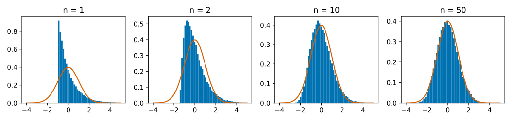
What the code does. For n = 1, 2, 10, 50 it generates 50,000 samples of n exponentials, computes their mean and standardises it with the CLT formula (z). The histogram (blue bars) is compared with the standard normal density (orange line). For n = 1 the shape is the exponential one, strongly asymmetric (skewness 2); with n = 50 it is almost a bell, with skewness 0.285. The fraction of values within ±1.96 is already 0.947 for n = 1 and 0.951 for n = 50: the 95% coverage is a weak property, which is not enough to declare a distribution normal, and this is why it matters to look at the skewness and the histogram as well. The skewness is a number that measures how much a distribution leans to one side: 0 for a symmetric one.

Trade-off and limits. The CLT is an asymptotic theorem: it says how it goes for n → ∞, not how large n must be. For almost symmetric distributions a few dozen observations are enough; for very asymmetric distributions or with heavy tails many more may be needed. It is the justification of what you will do in the statistics lesson: confidence intervals and tests based on the normal.

When it does not work: heavy tails

The CLT and the law of large numbers require a finite mean (and variance). The Cauchy distribution (the ratio of two standard normals) is an example in which they do not exist: the tails are so heavy that the extreme values dominate every mean.

rng = np.random.default_rng(2)
cauchy = rng.standard_cauchy(size=1_000_000)
normale = rng.standard_normal(size=1_000_000)
print("   n | Cauchy sample mean | normal sample mean")
for n in (100, 1_000, 10_000, 100_000, 1_000_000):
    print(f"{n:>7} | {cauchy[:n].mean():18.4f} | {normale[:n].mean():18.4f}")
print("maximum absolute value observed in the Cauchy:", round(float(np.abs(cauchy).max()), 1))

Output obtained:

   n | Cauchy sample mean | normal sample mean
    100 |            -2.1549 |            -0.0755
   1000 |            -1.8108 |            -0.0322
  10000 |             0.2042 |            -0.0100
 100000 |             0.6581 |             0.0006
1000000 |            -0.3914 |             0.0016
maximum absolute value observed in the Cauchy: 159848.9

What the code does. It computes the mean of the first n values of two samples. The normal one tends to zero as expected from the law of large numbers (from −0.08 with 100 values to 0.0016 with a million, irregularly because the mean is itself random). The Cauchy one does not converge: it oscillates between about −2 and +1 and changes sign irregularly even with a million values, because every now and then a gigantic value appears (here almost 160,000) that drags the mean. It is a known fact that the mean of n standard Cauchys is itself a standard Cauchy: averaging concentrates nothing. Adding data does not help.

Practical lesson. For data with heavy tails (amounts, response times, sizes) the mean can be an unstable summary: one uses the median and the quantiles, and always checks the histogram (visualisation lesson). Do not trust a mean without having looked at the tails.

Covariance and correlation

For two variables the covariance measures whether they tend to move together:

Cov(X, Y) = E[(X − μ_X)(Y − μ_Y)] = E[XY] − E[X]·E[Y].

Positive: they grow together; negative: one grows when the other falls. It depends on the units, so it is normalised into the correlation ρ = Cov(X, Y)/(σ_X σ_Y), always between −1 and +1. If X and Y are independent, E[XY] = E[X]E[Y] and Cov = 0. The converse is false: zero correlation does not mean independence, because it measures only the linear relationship.

rng = np.random.default_rng(8)
x = rng.normal(size=200_000)
y = x ** 2                                            # y is a function of x, hence dependent
print("corr(X, X^2) =", round(float(np.corrcoef(x, y)[0, 1]), 4), "(close to zero, but y = x^2 !)")

z = 0.8 * x + 0.6 * rng.normal(size=x.size)
print("corr(X, 0.8X + noise) =", round(float(np.corrcoef(x, z)[0, 1]), 4), "| theory 0.8")

Output obtained:

corr(X, X^2) = 0.0005 (close to zero, but y = x^2 !)
corr(X, 0.8X + noise) = 0.8012 | theory 0.8

What the code does. The first pair shows a perfect dependence (y is determined by x) with almost zero correlation: the relationship is a parabola, not a line, and the sign of x compensates. The second pair builds a linear relationship with noise; the coefficient 0.8 is exactly the theoretical correlation, because 0.8² + 0.6² = 1 keeps the variance of z equal to 1.

Typical mistakes (symptom, cause, remedy)

• "Mean = typical value". With asymmetric or heavy-tailed distributions the mean is far from the typical case. Remedy: median, quantiles, histogram.
• Adding standard deviations instead of variances. σ_{X+Y} = √(σ_X² + σ_Y²) for independent variables, not σ_X + σ_Y.
• Using the binomial without independence. If the trials depend (customers of the same family), the variance is not np(1−p).
• Confusing density and probability. A density can be 3 without violating anything: the area counts.
• Applying the CLT to small samples or heavy tails. Remedy: simulate, or use the bootstrap.
• Zero correlation = independence. False (parabola).
• Forgetting to fix the seed. The numbers change at every run.

The common thread is that every numerical summary (mean, standard deviation, correlation) hides a shape. The mistakes about the mean, the CLT and the correlation come from looking at the number without looking at the distribution that produced it; those about adding standard deviations and about density are formula mistakes, avoided by writing the calculations with the units of measure beside them; the one about the binomial is an assumption (independence) taken for granted.

How to work in practice

Choose the distribution from the mechanism that generates the data: count of successes in independent trials, binomial; rare events in an interval, Poisson; waiting times, exponential; sums of many small contributions, normal. Verify with a simulation every formula you need, always report mean and standard deviation together with the sample size n, look at the plot before choosing a summary and, for CDF, quantiles and sampling, use scipy.stats instead of hand-written formulas.

The vocabulary boils down to this. The random variable associates a number with each outcome; the PMF gives the mass of the discrete ones, the density describes the continuous ones and the CDF holds for both. The expected value is the mean weighted with the probabilities, the variance the squared dispersion around the mean and the standard deviation its root. The standardisation (X − μ)/σ brings any variable to mean 0 and standard deviation 1; asymptotic means valid in the limit n → ∞; heavy tails are distributions in which extreme values have non-negligible probability.

Mini-project

1. Simulate 100,000 times the number of heads in 30 tosses of a coin with p = 0.4. Compare mean, variance and observed frequencies with the binomial PMF.
2. With scipy.stats.poisson, verify that for λ = 4 the probability of obtaining at least 8 events equals 1 − F(7).
3. Verify by simulation the law of large numbers on a die: plot the mean of the first n rolls against n and add the band 3.5 ± 1.708/√n (the standard deviation of the die is 1.708).

The three points resemble each other: they compare a theoretical number, proved in the lesson, with an estimate by simulation. If the two values do not coincide within the expected noise (of the order of σ/√n), the first suspicion falls on the code and not on the theorem; the third point is developed in full in the worked challenge below.

A worked challenge: the law of large numbers on a die

The mini-project asked to verify the law of large numbers on a die, with an uncertainty band around the mean. The true mean is 3.5 and the standard deviation √(35/12) ≈ 1.708 (computed in this lesson); the mean of n rolls therefore has standard deviation 1.708/√n. If the law and the CLT work, about 95% of the sample means should fall inside 3.5 ± 1.96·1.708/√n.

import numpy as np

rng = np.random.default_rng(13)
sigma = np.sqrt(35 / 12)
lanci = rng.integers(1, 7, size=(5_000, 10_000))                 # 5000 independent series of 10,000 rolls
cumulata = np.cumsum(lanci, axis=1) / np.arange(1, lanci.shape[1] + 1)

print(f"{'n':>6} {'mean of the means':>18} {'observed std. dev.':>19} {'sigma/sqrt(n)':>14} {'share inside 3.5±1.96·σ/√n':>28}")
for n in (10, 100, 1_000, 10_000):
    medie_n = cumulata[:, n - 1]
    teorica = sigma / np.sqrt(n)
    dentro = (np.abs(medie_n - 3.5) <= 1.96 * teorica).mean()
    print(f"{n:>6} {medie_n.mean():>18.4f} {medie_n.std():>19.4f} {teorica:>14.4f} {dentro:>28.3f}")

Output obtained:

     n  mean of the means  observed std. dev.  sigma/sqrt(n)   share inside 3.5±1.96·σ/√n
    10             3.4934              0.5458         0.5401                        0.952
   100             3.4982              0.1726         0.1708                        0.949
  1000             3.4997              0.0544         0.0540                        0.949
 10000             3.5001              0.0172         0.0171                        0.947

How to read the code. lanci is a 5000 × 10,000 matrix: each row is a series of rolls of a fair die (rng.integers(1, 7, ...) draws integers from 1 to 6). np.cumsum(..., axis=1) computes, for each series, the running sum of the rolls; dividing by 1, 2, 3, … (the number of rolls made up to that point) gives the running mean: column n − 1 contains the mean of the first n rolls of each series. For four values of n three things are compared: the mean of the 5000 means (which must be close to 3.5), the observed standard deviation of the means (which must follow σ/√n: one divides by √10 ≈ 3.16 each time n is multiplied by 10) and the share of means inside the two-sigma band, close to the 95% predicted by the CLT. The fact that the two columns observed std. dev. and sigma/sqrt(n) coincide is the experimental verification of Var(X̄) = σ²/n.

Challenge

• Easy. Compute by hand E[X] and Var(X) for a variable taking 0, 1, 2 with probabilities 0.5, 0.3, 0.2 and verify in code.
• Medium. Prove that for a Poisson E[X] = λ: Σ k e^(−λ) λᵏ/k! = λ Σ e^(−λ) λ^(k−1)/(k−1)! = λ.
• Hard. Prove Var(aX + b) = a²Var(X) and verify with 100,000 normal samples with a = 3, b = 5.
• Expert. Prove that for any two variables Var(X + Y) = Var(X) + Var(Y) + 2Cov(X, Y), and use the result to explain why the variance of the mean of n correlated variables does not fall as σ²/n.
• Enterprise. Take the series of response times of a service in your organisation: is the exponential a good model? Compare mean and median, the memoryless property, and declare whether the mean is a safe summary.

The first three challenges are guided calculations on the formulas of the lesson, the fourth tests covariance, the fifth asks for a judgement on real data: if the median of your response times is much lower than the mean, the long tail you saw with the Cauchy is already at work in your data.

What you can do now

You can associate a number with every outcome, compute expected value and variance with linearity and with the formula "mean of the squares minus square of the mean", choose among binomial, Poisson, exponential and normal according to the mechanism, and verify by simulation the law of large numbers and the central limit theorem. You can also recognise when they do not hold: with a Cauchy the mean does not converge, and averaging concentrates nothing. The next step is statistics, which travels the opposite road from data to parameters, with the integrals of densities explained in Calculus 2.

The same series also includes: 29 - Sampling and Monte Carlo Methods: Estimating What You Cannot Compute (which refers back to this lesson).