You have computed the mean, the standard deviation and the correlation of a sample, and the numbers look reasonable. The question is how far you can trust them. A summary number compresses tens or thousands of values into one, and what it throws away depends on the data: two very different samples can produce the same summary. A chart gives back the lost information, which is why you draw it before computing and modelling, not at the end of the analysis as decoration. In this lesson of the "Python for data" module you build charts with Matplotlib explicitly (Figure and Axes), choose the type of chart according to the question, set the bins of a histogram by a criterion instead of by eye, measure how much a truncated axis deceives, and see with four small datasets why statistics alone are not enough.
You need Python 3, NumPy and Matplotlib (pip install numpy matplotlib in a virtual environment). The listings were run with Python 3.14.4, NumPy 2.3.5 and Matplotlib 3.10.7; where a function changes from one version to another I say so. If you come from the lesson on Pandas, remember that DataFrame.plot is a wrapper around Matplotlib: what you learn here also holds for charts that start from a table.
The anatomy of Matplotlib
The frame and the picture
The Figure is the whole canvas, the frame: the object you save to a file. Inside you can hang one or more pictures, and each one is an Axes. The name is plural but it denotes one panel with its axes, not "the axes". The line with numbers along one side is an Axis, and everything that gets drawn (lines, points, texts) is an Artist. Confusing Axes with Axis is the most common vocabulary mistake, and it makes the documentation hard to read.
Matplotlib offers two ways of using it. The first, with global state, goes through the pyplot functions such as plt.plot(...) and plt.title(...): they work on "the current figure", and in a notebook for a quick chart they are perfectly fine; with several figures open, however, you lose track of which one is current. The second is the object interface: you ask for fig, ax = plt.subplots() and then call the methods of ax, so you always know which panel you are drawing on. It is more verbose and more explicit, and the Matplotlib quick start guide describes the two styles as the two possible roads, pointing to the API page for the trade-offs. In this lesson we use the second, because code that has to last and pass from one function to another needs to know which ax it is writing on.
The listing draws sine and cosine on the same panel. Two lines deserve attention: matplotlib.use("Agg"), which chooses the non-interactive backend (the drawing engine), the one that writes only to files and also works on a server without a screen; and plt.rcParams["svg.hashsalt"] together with metadata={"Date": None}, which serve only to make the SVG file identical byte for byte at every run (otherwise Matplotlib embeds a random identifier and the date). In everyday code you do not need them.
import numpy as np
import matplotlib
matplotlib.use("Agg")                       # non-interactive backend: writes only to files
import matplotlib.pyplot as plt

plt.rcParams["svg.hashsalt"] = "mle"           # SVGs reproducible byte for byte
x = np.linspace(0, 2 * np.pi, 200)

fig, ax = plt.subplots(figsize=(6, 3))
ax.plot(x, np.sin(x), label="sin(x)")
ax.plot(x, np.cos(x), label="cos(x)", linestyle="--")
ax.set_xlabel("x (radians)")
ax.set_ylabel("value")
ax.set_title("Two functions on the same panel")
ax.legend()
fig.tight_layout()
fig.savefig("sine-cosine.svg", metadata={"Date": None})
plt.close(fig)
print("figure saved:", type(fig).__name__, "| axes:", type(ax).__name__, "| backend:", matplotlib.get_backend())
Output obtained (Python 3.14.4, NumPy 2.3.5, Matplotlib 3.10.7; the listing was run twice with identical output):
figure saved: Figure | axes: Axes | backend: Agg
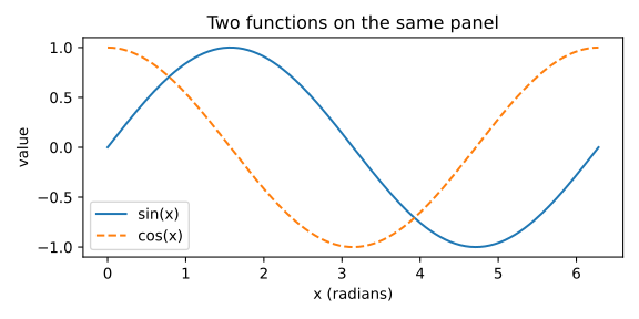
The output confirms the types: plt.subplots returns a Figure object and an Axes, and the backend in use is Agg. Without the matplotlib.use line, on my machine the backend chosen automatically was qtagg, one of the interactive ones: it is one of the reasons why the same script can behave differently on two machines. Three more notes. plt.close(fig) frees the memory of the figure: in a loop that creates hundreds of them, forgetting it accumulates them, and Matplotlib reports the problem beyond 20 open figures (figure.max_open_warning is 20, measured in the last listing of the lesson). savefig chooses the format from the extension: a vector format (svg, pdf) stays sharp at any magnification, while png with a suitable dpi= is better for figures with millions of points. Finally, writing to a file is writing to a file: if the path does not exist or the folder is not writable you get the same errors you meet with any other file, described in the lesson on functions, files, exceptions and objects.
Which chart for which question
The basic rule, valid for any library, is first the question, then the chart. The table pairs the five questions you meet most often with the chart that serves them best and the reason.
| The question | The chart | Why |
|---|---|---|
| How are the values distributed? | histogram, boxplot, empirical distribution function | shows shape, centre, spread, tails, peaks |
| Is there a relationship between two numbers? | scatter plot | each point is a case; you see the cloud |
| How does it change over time? | line chart | the line conveys continuity and direction |
| Which category is bigger? | bars (horizontal if the labels are long) | the length from a common baseline can be compared precisely |
| How much does each part weigh? | stacked bars or simple sorted bars | pie slices are hard to compare |
Behind the table there is an experimental result: Cleveland and McGill (1984) measured how accurately people read different graphical elements and found that position along a common scale (points, bars from the same baseline) is judged better than angle, area or colour. That is why bars beat pies when the task is to compare. The trade-off is always the same: a richer chart, with colour for a third variable and the size of the point for a fourth, conveys more information but costs more reading effort. Every extra visual element must answer one more question; otherwise remove it.
The same sample with three charts
The histogram is not the only way to look at a distribution, and for data with long tails or outliers it is not the best. The next listing generates 500 response times from a log-normal distribution (which has a right tail, like real times) and adds three outliers to it, 14, 17.5 and 22 seconds. Then it draws them with a histogram, a boxplot (box and whiskers) and an empirical distribution function, ECDF. The seed of the generator (default_rng(5)) fixes the sample: two runs give the same numbers. A version note: in the boxplot the orientation is chosen with orientation="horizontal", introduced in Matplotlib 3.10; the old vert=False argument is marked as deprecated from 3.11 in the current documentation, so I do not use it.
import numpy as np
import matplotlib
matplotlib.use("Agg")
import matplotlib.pyplot as plt

plt.rcParams["svg.hashsalt"] = "mle"
rng = np.random.default_rng(5)
tempi = np.concatenate([rng.lognormal(mean=0.0, sigma=0.6, size=500), [14.0, 17.5, 22.0]])

q1, mediana, q3 = np.percentile(tempi, [25, 50, 75])
print(f"mean = {tempi.mean():.2f} | median = {mediana:.2f} | interquartile range = {q3 - q1:.2f} | maximum = {tempi.max():.1f}")

fig, assi = plt.subplots(1, 3, figsize=(11, 3))
assi[0].hist(tempi, bins=40, color="#0072B2", edgecolor="white")
assi[0].set_title("histogram")
assi[1].boxplot(tempi, orientation="horizontal", widths=0.5)
assi[1].set_title("boxplot")
ordinati = np.sort(tempi)
assi[2].step(ordinati, np.arange(1, ordinati.size + 1) / ordinati.size, color="#D55E00")
assi[2].set_title("ECDF")
for ax in assi:
    ax.set_xlabel("response time (s)")
fig.tight_layout()
fig.savefig("three-views.svg", metadata={"Date": None})
plt.close(fig)
Output obtained (Python 3.14.4, NumPy 2.3.5, Matplotlib 3.10.7; the listing was run twice with identical output):
mean = 1.28 | median = 0.99 | interquartile range = 0.86 | maximum = 22.0
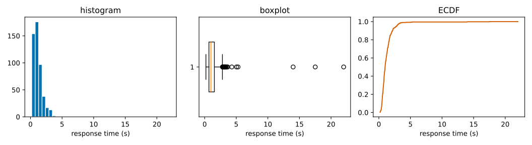
The printed numbers already say a lot: the mean (1.28) exceeds the median (0.99) by almost three tenths because the three outliers drag it upwards, while the interquartile range, the width of the central 50% of the data, stays 0.86. In the histogram the shape is there, but the three outliers are almost invisible: columns one element tall, very far from the rest. The boxplot draws the box between the first and third quartile with a line on the median; according to the documentation of Axes.boxplot the whiskers reach the farthest datum lying within 1.5 times the interquartile range from the box, and the points beyond the whiskers are drawn one by one: here the outliers jump out. The ECDF (for each value x, the fraction of data less than or equal to x) does not depend on any bin choice and is read vertically on the quantiles: where the curve crosses 0.5 there is the median. Three tools, three questions: the shape, the outliers, the quantiles without arbitrariness.
Histograms: how many bins?
A histogram divides the axis into intervals of equal width, the bins, and counts how many data fall in each. The only parameter that matters is the width, and the choice is a compromise. With bins that are too wide everything is squashed and the structures disappear: that is the distortion (bias). With bins that are too narrow each column contains few data, the profile becomes jagged and invents peaks that do not exist: that is the noise, that is the variance. It is the same trade-off between simplifying too much and chasing the noise that you find again throughout machine learning, for instance when you choose the complexity of a model.
To avoid going by eye there are rules that fix the number or the width of the bins, and NumPy implements them all in numpy.histogram_bin_edges (the bins argument with the name of the method). With n data: the Sturges rule (1926) uses k = ⌈log₂ n⌉ + 1 bins and takes into account only n; the Scott rule (1979) uses the width h = 3.49 · σ · n-1/3, with σ the standard deviation; the Freedman and Diaconis rule (1981) uses h = 2 · IQR · n-1/3, with IQR the interquartile range. The factor n-1/3 comes from minimising the integrated mean squared error of the histogram as a density estimate, which adds a bias term (growing with the width) and a variance term (falling with the width); the optimal width balances them. Scott's constant 3.49 coincides with the (24·√π)1/3 you find in NumPy's code, and Sturges's, in NumPy's implementation, is the width "range of the data divided by log₂ n + 1" (I read it in the source of the installed version).
An option worth knowing is "auto": according to the documentation it takes the minimum width between that of Sturges and that of Freedman-Diaconis. When you indicate nothing, np.histogram uses 10 bins instead (measured at the end of the lesson).
Let us see the compromise on data with two groups: 300 points around 0 and 300 around 4, generated with a fixed seed. The listing prints the number of bins chosen by each method and then draws the same sample with 2, 11 and 200 bins.
import numpy as np
import matplotlib
matplotlib.use("Agg")
import matplotlib.pyplot as plt

plt.rcParams["svg.hashsalt"] = "mle"
rng = np.random.default_rng(3)
dati = np.concatenate([rng.normal(0, 1, 300), rng.normal(4, 1, 300)])

for metodo in ("sturges", "fd", "scott"):
    k = len(np.histogram_bin_edges(dati, bins=metodo)) - 1
    print(f"{metodo:8s}: {k} bins")

fig, assi = plt.subplots(1, 3, figsize=(10, 2.8), sharey=False)
for ax, k in zip(assi, (2, 11, 200)):
    ax.hist(dati, bins=k, color="#0072B2", edgecolor="white")
    ax.set_title(f"{k} bins")
    ax.set_xlabel("value")
assi[0].set_ylabel("count")
fig.tight_layout()
fig.savefig("histograms-bins.svg", metadata={"Date": None})
plt.close(fig)
Output obtained (Python 3.14.4, NumPy 2.3.5, Matplotlib 3.10.7; the listing was run twice with identical output):
sturges : 11 bins
fd      : 11 bins
scott   : 11 bins
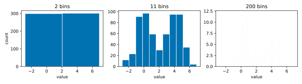
The three rules all give 11 bins on this sample: with 600 points Sturges computes ⌈log₂ 600⌉ + 1 = 11, and the two based on dispersion arrive by chance at the same number because the data are two Gaussians of equal width. It is not a general rule, as you will see shortly. The comparison that matters is visual: with 2 bins you see a single block, and the two groups do not exist; with 200 bins you see a dust; with 11 two distinct hills emerge, with a few irregular steps that are the noise of the sample. No rule replaces the eye, and it is a good habit to try two or three values and check that the story does not change. In the code, plt.subplots(1, 3) creates a row of three Axes and returns an array to loop over with zip; edgecolor="white" separates the columns.
What happens to the bins when outliers arrive
The three rules do not react in the same way to extreme values, and this is the reason why Freedman-Diaconis is considered the most robust (NumPy's documentation describes it as "resilient to outliers"). The listing takes 1000 normal points, adds five enormous outliers (from 50 to 90) and compares the bin widths of the three rules on the clean sample and on the dirty one. The widths are read directly from the edges returned by histogram_bin_edges. In the same listing, at the end, are the two measurements cited earlier: the default number of bins of np.histogram and the value of figure.max_open_warning.
import numpy as np
import matplotlib
matplotlib.use("Agg")
import matplotlib.pyplot as plt

rng = np.random.default_rng(1)
dati = rng.normal(0, 1, 1000)
sporchi = np.concatenate([dati, [50.0, 60.0, 70.0, 80.0, 90.0]])
for etichetta, campione in (("clean", dati), ("with 5 outliers", sporchi)):
    larghezze = []
    for metodo in ("sturges", "scott", "fd"):
        bordi = np.histogram_bin_edges(campione, bins=metodo)
        larghezze.append(f"{metodo}={bordi[1] - bordi[0]:.3f}")
    print(f"{etichetta:16s}", " | ".join(larghezze))
print("default bins of np.histogram:", np.histogram(dati)[0].size, "| rcParams max_open_warning:", plt.rcParams["figure.max_open_warning"])
Output obtained (Python 3.14.4, NumPy 2.3.5, Matplotlib 3.10.7; the listing was run twice with identical output):
clean            sturges=0.664 | scott=0.332 | fd=0.261
with 5 outliers  sturges=8.504 | scott=1.765 | fd=0.267
default bins of np.histogram: 10 | rcParams max_open_warning: 20
On the clean sample the widths are 0.664 (Sturges), 0.332 (Scott) and 0.261 (Freedman-Diaconis). With five outliers Sturges jumps to 8.504, because its width is the range of the data divided by a number of bins that depends only on n, and the range has become enormous: all the real data end up in one or two bins. Scott rises to 1.765, because the standard deviation squares the deviations and the outliers inflate it. Freedman-Diaconis goes from 0.261 to 0.267: the interquartile range looks only at the central 50% and the outliers do not move it. The price of this robustness is that, if the outliers are the interesting part of the data, the resulting bin does not cover them: they must be found with another chart, the boxplot, which is made for that.
Exercise 1
How many bins, and why exactly those
A bakery weighs the loaves coming out of its two ovens. Apply the three formulas of the previous section, pen and paper: the numbers are chosen so that the calculations come out exact.
- With
n = 256weighings, how many bins does Sturges suggest? Why is the result an exact integer? - With
n = 1000weighings and an interquartile range of15 g, what is the Freedman-Diaconis width? Why is the calculation exact here too? - With the same
n = 1000and a standard deviation of20 g, what is Scott's width? If you added three defective loaves of 2 kg, which of the two widths would change more?
Before opening the solution try to answer at least the first two questions: they need only a power of two and a cube root of a thousand, and if the calculations do not add up it is worth rereading the formulas in the section on histograms.
Show the solution
1. k = ⌈log₂ 256⌉ + 1 = 8 + 1 = 9 bins. It is exact because 256 = 2⁸: the base-2 logarithm is 8 with no rounding, and the ceiling has nothing to round.
2. h = 2 · IQR · n^(-1/3) = 2 · 15 · (1/10) = 3.0 g. Exact because 1000 = 10³, hence n^(-1/3) = 1/10 exactly.
3. h = 3.49 · 20 · 0.1 = 6.98 g, more than double. The two rules measure the dispersion in different ways: Scott uses the standard deviation, Freedman-Diaconis the interquartile range. Three loaves of 2 kg among a thousand of half a kilo would greatly inflate the standard deviation, which squares the deviations, and would leave the interquartile range almost still, since it looks only at the central 50% of the data. So Scott's width changes more; it is the same effect that the previous listing measured with five outliers.
Axes that deceive
In a chart of bars the information lies in the length. If the axis does not start from zero, the length stops being proportional to the value and the differences swell. Tufte (1983) gave a name to the measure of the deception, the lie factor: the size of the effect shown in the chart divided by the size of the effect in the data. An honest chart is worth 1. The listing takes two values, 100 and 104, computes the true difference (4%), computes the difference the eye sees if the axis starts from 98 (the bars become 2 and 6 long) and divides them. It then draws the same bars with the two axes. I use horizontal bars (barh): the length encodes the value in the same way, and only the axis to be truncated changes, which is the horizontal one (set_xlim).
import numpy as np
import matplotlib
matplotlib.use("Agg")
import matplotlib.pyplot as plt

plt.rcParams["svg.hashsalt"] = "mle"
valori = np.array([100.0, 104.0])

effetto_dati = (valori[1] - valori[0]) / valori[0]              # 4 %
base_taglio = 98.0
altezze_viste = valori - base_taglio                            # 2 and 6
effetto_grafico = (altezze_viste[1] - altezze_viste[0]) / altezze_viste[0]
print(f"difference in the data  : {effetto_dati:.1%}")
print(f"difference seen by eye  : {effetto_grafico:.1%}")
print(f"lie factor              : {effetto_grafico / effetto_dati:.0f}")

fig, assi = plt.subplots(1, 2, figsize=(7, 3))
for ax, base, titolo in zip(assi, (98, 0), ("axis from 98: deceives", "axis from 0: honest")):
    ax.barh(["A", "B"], valori, color=["#56B4E9", "#D55E00"])
    ax.set_xlim(base, 106)
    ax.set_title(titolo)
fig.tight_layout()
fig.savefig("misleading-axes.svg", metadata={"Date": None})
plt.close(fig)
Output obtained (Python 3.14.4, NumPy 2.3.5, Matplotlib 3.10.7; the listing was run twice with identical output):
difference in the data  : 4.0%
difference seen by eye  : 200.0%
lie factor              : 50
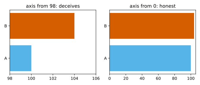
A 4% difference appears as triple the length: the eye sees an increase of 200% and the lie factor is 50. For bars the axis starts from zero, always. For a line chart the argument changes: the line encodes position, not length from a baseline, and an axis that does not start from zero can be legitimate to show a trend; the obligation remains to declare the interval and not to compare the slopes of charts with different scales. There are other ways of deceiving, even unintentionally: a double vertical axis (the apparent correlation depends on the choice of the two scales), three-dimensional charts with perspective (depth alters the areas), pies with too many slices, undeclared non-linear scales.
Exercise 2
How much this figure lies
The bakery's monthly report compares two days with a chart of bars: 250 and 260 loaves baked. The vertical axis starts from 240.
- What is the change present in the data, as a percentage?
- How tall are the two bars on the page, and by what percentage does the height change?
- Compute the lie factor. What would happen if the axis started from
250?
The procedure is identical to that of the listing in the previous section: first the effect in the data, then the effect on the page after removing the base of the axis, finally the ratio between the two. Follow the same three steps with the bakery's numbers.
Show the solution
1. (260 - 250) / 250 = 0.04, that is 4%.
2. The visible heights are 250 - 240 = 10 and 260 - 240 = 20: the second is twice as tall as the first, a change of 100%.
3. 100% / 4% = 25. An honest chart is worth 1; this one multiplies by twenty-five the effect the reader perceives. With the axis at 250 the first would have height zero, the relative change would not even be defined and the factor would be infinite: the figure would turn "4% more" into "exists versus does not exist".
Anscombe's quartet
In 1973 Francis Anscombe published four small datasets, of 11 pairs (x, y) each, built to have the same summary statistics. He wanted to refute the idea that calculations are enough and that the chart is a useless decoration. In the listing the four sets are in a dictionary of tuples, the structure described in the lesson on lists, tuples, dictionaries and sets; for each one it prints the means, the variance of y (with ddof=1, the sample variance), the Pearson correlation (np.corrcoef) and the coefficients of the least-squares line (np.polyfit(x, y, 1), which returns slope and intercept). Then a 2×2 grid with shared axes (sharex=True, sharey=True, to make the four charts directly comparable) draws the points and the line.
import numpy as np
import matplotlib
matplotlib.use("Agg")
import matplotlib.pyplot as plt

plt.rcParams["svg.hashsalt"] = "mle"
x1 = np.array([10, 8, 13, 9, 11, 14, 6, 4, 12, 7, 5], dtype=float)
x4 = np.array([8, 8, 8, 8, 8, 8, 8, 19, 8, 8, 8], dtype=float)
quartetto = {
    "I":   (x1, np.array([8.04, 6.95, 7.58, 8.81, 8.33, 9.96, 7.24, 4.26, 10.84, 4.82, 5.68])),
    "II":  (x1, np.array([9.14, 8.14, 8.74, 8.77, 9.26, 8.10, 6.13, 3.10, 9.13, 7.26, 4.74])),
    "III": (x1, np.array([7.46, 6.77, 12.74, 7.11, 7.81, 8.84, 6.08, 5.39, 8.15, 6.42, 5.73])),
    "IV":  (x4, np.array([6.58, 5.76, 7.71, 8.84, 8.47, 7.04, 5.25, 12.50, 5.56, 7.91, 6.89])),
}

print("set     | mean x  | mean y  | var y | corr  | slope    | intercept")
for nome, (x, y) in quartetto.items():
    pend, interc = np.polyfit(x, y, 1)
    r = np.corrcoef(x, y)[0, 1]
    print(f"{nome:7s} | {x.mean():7.2f} | {y.mean():7.2f} | {y.var(ddof=1):5.2f} | {r:5.3f} | {pend:8.3f} | {interc:9.2f}")

fig, assi = plt.subplots(2, 2, figsize=(7, 5), sharex=True, sharey=True)
retta_x = np.array([3, 20])
for ax, (nome, (x, y)) in zip(assi.ravel(), quartetto.items()):
    pend, interc = np.polyfit(x, y, 1)
    ax.scatter(x, y, color="#0072B2")
    ax.plot(retta_x, pend * retta_x + interc, color="#D55E00")
    ax.set_title(f"Set {nome}")
fig.tight_layout()
fig.savefig("anscombe-en.svg", metadata={"Date": None})
plt.close(fig)
Output obtained (Python 3.14.4, NumPy 2.3.5, Matplotlib 3.10.7; the listing was run twice with identical output):
set     | mean x  | mean y  | var y | corr  | slope    | intercept
I       |    9.00 |    7.50 |  4.13 | 0.816 |    0.500 |      3.00
II      |    9.00 |    7.50 |  4.13 | 0.816 |    0.500 |      3.00
III     |    9.00 |    7.50 |  4.12 | 0.816 |    0.500 |      3.00
IV      |    9.00 |    7.50 |  4.12 | 0.817 |    0.500 |      3.00
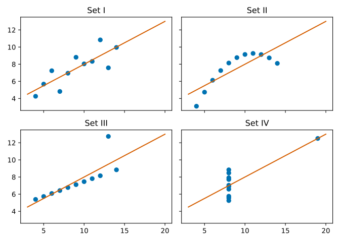
The table says that the four sets are, to two or three decimals, the same thing: means 9.00 and 7.50, correlation 0.816 (0.817 for IV), line y ≈ 3 + 0.5·x. The chart tells four stories. Set I is a cloud with a plausible linear relationship, and the line describes it well. II is a curve: the relationship is not linear and the line is the wrong model. In III the points lie on an almost perfect line, and a single anomalous point tilts it and lowers the correlation. In IV x is constant in ten cases out of eleven, so in the large group there is no relationship between x and y, and a single isolated point creates all the correlation by itself. The values are those of the original work, transcribed by me by hand from a source I could not open (see the end); that the statistics coincide you can verify yourself in the output above. The operational lesson: correlation is a summary that holds only if the shape of the relationship is the one assumed. Before trusting a correlation, a regression or a mean, look at the data.
Too many points: overplotting
With a scatter plot of many thousands of points, the points overlap and the chart becomes a uniform blob where density cannot be read. The classic remedies are two: make the points transparent (alpha), so the dense zones come out darker, or count the points in hexagonal cells and colour by density (hexbin). The listing generates 30,000 points with a linear relationship plus noise and draws them in the three ways; mincnt=1 hides the empty hexagons, as described in the documentation of Axes.hexbin, and fig.colorbar adds the scale of the counts.
import numpy as np
import matplotlib
matplotlib.use("Agg")
import matplotlib.pyplot as plt

plt.rcParams["svg.hashsalt"] = "mle"
rng = np.random.default_rng(9)
n = 30_000
x = rng.normal(0, 1, n)
y = 0.6 * x + rng.normal(0, 0.8, n)
print("correlation of the data:", round(float(np.corrcoef(x, y)[0, 1]), 3), "| points:", n)

fig, assi = plt.subplots(1, 3, figsize=(11, 3.2), sharex=True, sharey=True)
assi[0].scatter(x, y, s=6, color="#0072B2")
assi[0].set_title("simple scatter")
assi[1].scatter(x, y, s=6, color="#0072B2", alpha=0.05)
assi[1].set_title("alpha = 0.05")
esagoni = assi[2].hexbin(x, y, gridsize=35, cmap="viridis", mincnt=1)
assi[2].set_title("hexbin")
fig.colorbar(esagoni, ax=assi[2], label="points per cell")
fig.tight_layout()
fig.savefig("overplotting-en.svg", metadata={"Date": None})
plt.close(fig)
Output obtained (Python 3.14.4, NumPy 2.3.5, Matplotlib 3.10.7; the listing was run twice with identical output):
correlation of the data: 0.593 | points: 30000

The correlation of the data is 0.593. In the first panel 30,000 opaque points form a blue blob: you understand that there is a cloud but not where it is denser. In the second, with alpha=0.05 (95% transparency for each point), the points add up and the dense zones appear darker: the elliptical shape and the thicker centre emerge. In the third the hexbin counts how many points fall in each hexagon and colours them with viridis. The point is not aesthetic: with large quantities of data, a chart that shows only the single points hides the distribution. To choose the two parameters, alpha and gridsize, there is no formula: you try a few values until the structure you see survives a small change.
Colours, labels, accessibility
A correct chart can still be unreadable. Two rules of common sense: always label axes and units ("value" says nothing, "temperature (°C)" does), and write a title that states the conclusion ("sales grow by 12% in April") instead of the type of chart. Colour needs more attention. A page by Okabe and Ito devoted to Color Universal Design reports that about one man in twelve among people of Caucasian origin (8%) has red-green colour blindness, one in twenty among Asians (5%), one in twenty-five among Africans (4%): in a room of 250 people there are more than ten. Red and green are the pair most often confused, and for this reason they must not be the only difference between two series. In the figures of this lesson I use the colours of the Okabe and Ito palette (#0072B2, #D55E00, #56B4E9, taken from the widespread hexadecimal transcription of their palette; the page presents it as an image, so I did not reread the values from text). Do not rely on colour alone either: add marker shape or line style, because the figure might be printed in black and white.
For colour maps that represent an intensity the Matplotlib guide to choosing colormaps recommends perceptually uniform maps, in which equal steps in the data are perceived as equal steps in colour: viridis, the default map, is one of these. The same page shows that jet has a luminosity that varies irregularly along the scale, and is a poor choice for representing data; the practical effect is that bands appear in the rainbow that the eye reads as differences that are not in the data.
Typical errors
| Symptom | Cause | Remedy |
|---|---|---|
| Two bars look very different, and the data do not | truncated axis on a chart of bars | axis from zero; to magnify a difference use a dot plot with the uncertainty interval |
| The histogram changes shape as the bins change | it is not a bug: it is the trade-off between bias and noise | try several values and show only what survives |
| A black cloud in which nothing can be seen | too many overlapping points | low alpha=, small markers, hexbin or ax.hist2d |
| Memory grows in a loop of figures | plt.close forgotten |
always close the figure after savefig |
| The chart is different on different machines | backend, fonts or library version | fix the backend, save in a vector format, declare the versions |
| The chart seems to prove a cause | a cloud of points shows association, not causation | say so in the title and in the text; the cause is argued outside the chart |
Almost all these rows have the same root: the chart makes the data say something they do not say, through a choice of scale, bins or overlap made without looking at its effect. The defence is the same in every case: change the choice and check that the conclusion still stands.
Before handing over a figure
- Draw before computing, and again after modelling (the residuals, the predictions against the true values).
- Use the object interface and pass the
axto the drawing functions: the code stays reusable. - One figure, one message: if you need two, make two figures.
- Save from code, not with a screenshot, because the figure must be regenerable.
- Declare the data: where they come from, how many points, which period.
These five checks are independent of one another and you can apply them in the order you prefer; the first is the one most often skipped, and it is the one that would have made you notice the three outliers in the sample of response times, or the isolated point in the fourth Anscombe set, immediately.
Mini-project
Generate with NumPy, with a fixed seed, two normal samples of 500 points with means 0 and 0.3 and standard deviation 1, and work through the following steps.
- Draw the two overlapping histograms with
alpha=0.5and the same set of bins, computed only once withnp.histogram_bin_edgeson the merged data. - Compute the sample means and write in two lines whether from the chart alone you could tell that the means are different.
- Add two dashed vertical lines at the means.
- Save in
svgand inpngat 150 dpi and compare the file sizes.
Using the same bins for the two samples is the point of the first step: with different bins the visual comparison is no longer honest, because the columns are no longer counted on the same intervals. The second step forces you to reason about a question that statistics tackles formally with hypothesis tests: is a difference of 0.3 standard deviations visible by eye?
Challenges
- Easy. Reproduce the chart of bars with a truncated axis for three values (100, 101, 103) and compute the lie factor between the first and the last.
- Medium. Draw the empirical distribution function of a sample (sort the data and plot
i/nagainst the sorted value) and compare it with the histogram: which of the two does not depend on a choice of bins? - Hard. Build your own "quartet": two sets with the same mean and the same variance but a very different shape (for example one normal and one bimodal). Check with
np.mean,np.varand with the chart. - Expert. In the outliers listing, change the number and value of the outliers and observe how the widths of Sturges, Scott and Freedman-Diaconis grow. At what number of outliers does Freedman-Diaconis too begin to move, and why?
- Enterprise. Take an internal report of your organisation that contains a chart of bars or lines, measure the lie factor, check that the axes have units and rewrite the figure with a title that states the conclusion.
The Expert challenge has an answer you can predict: the interquartile range depends on the 75th percentile, so Freedman-Diaconis should move little as long as the outliers are a small fraction of the sample and jump when they exceed about a quarter. A test of mine (seed 1, 1000 normal points plus outliers all equal to 60) gave a width of 0.267 with 5 outliers, 0.290 with 100, 0.429 with 300 and 10.59 with 400: it goes in the predicted direction, but before trusting it repeat the test with your own numbers. If you did the Hard one, look at what the correlation of your quartet says, and compare it with Anscombe's.
In the next lesson, scikit-learn: estimators, pipelines and validation, you move from the array to the model, with the method for not fooling yourself: the separation between training data and test data.
The same series also includes: 11 - Floating-Point Numbers: Why 0.1 + 0.2 Is Not 0.3, 23 - Linear Algebra 1: Vectors, Matrices, Systems (which refer back to this lesson).
Sources
- Matplotlib, Quick start guide - the distinction between the object (explicit) style and the pyplot (implicit) style; consulted on 2026-11-12
- NumPy, numpy.histogram_bin_edges - description of the sturges, fd, scott and auto methods (fd as robust to outliers, auto as the minimum of sturges and fd); consulted on 2026-11-12
- Matplotlib, Axes.boxplot - whiskers within 1.5 times the interquartile range, orientation parameter; consulted on 2026-11-12
- Matplotlib, Axes.hexbin - meaning of mincnt; consulted on 2026-11-12
- Matplotlib, Choosing Colormaps in Matplotlib - perceptually uniform maps and the case of jet; consulted on 2026-11-12
- M. Okabe and K. Ito, Color Universal Design (CUD) - frequency of red-green colour blindness in males (8%, 5%, 4% per group); consulted on 2026-11-12
Bibliographic references cited in the text that I could not open (the publishers' sites answer 403 to automated requests, and I have not verified the pages): F. J. Anscombe, Graphs in Statistical Analysis, The American Statistician 27(1), 1973; E. R. Tufte, The Visual Display of Quantitative Information, Graphics Press, 1983; W. S. Cleveland and R. McGill, Graphical Perception, Journal of the American Statistical Association 79(387), 1984; H. A. Sturges, The Choice of a Class Interval, JASA 21(153), 1926; D. W. Scott, On Optimal and Data-Based Histograms, Biometrika 66(3), 1979; D. Freedman and P. Diaconis, On the Histogram as a Density Estimator: L2 Theory, 1981. What I report of them (the lie factor, the ranking of perceptual tasks, the three bin rules) is known in the literature, but the details were not reread on the original source.
Commenti
Caricamento commenti...
Sign in to comment