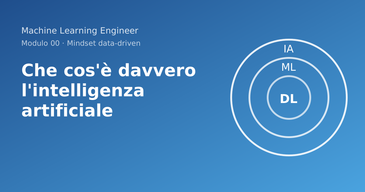
Machine Learning Engineer course · Module 00 · Data-driven mindset · Lesson 1
Goal. Give the reader a solid mental model of what AI is, where machine learning sits inside it, and why "learning from data" is an engineering technique and not magic. By the end the reader can tell a rule-based system from a learned one, can read the formal definition of learning, and knows why "it works on my dataset" is never enough.
Myth to dispel. "AI", "machine learning" and "deep learning" are synonyms. They are not: they are nested sets.
Introduction
This is the first lesson of the course. I will take you from "I have heard of AI" to "I can build, evaluate and deploy a model". The path is linear: first the way of thinking (module 00), then the tools (Python, module 01), then the mathematics that holds everything up (module 02), then the models.
End result of this lesson. You will be able to explain in three sentences what separates a traditional program from a learned one, and you will have run on your own computer an experiment that proves it with numbers.
Roadmap of the lesson.
- Programming versus learning (the central idea).
- The formal definition, in full, without skipping steps.
- The matryoshka dolls: AI ⊃ ML ⊃ DL.
- The three ways of learning.
- Generalising: the difference between memorising and understanding.
- When machine learning is the wrong choice.
The order is not random: the formal definition rests on the idea of a learned program, the AI-ML-DL hierarchy and the three paradigms use it as vocabulary, and the section on limits only makes sense after you have seen what ML can do. If you are in a hurry, read at least the first and the last item: they are the ones that change the decisions of a project.
What it is, why it exists, when NOT to use it
The problem AI tries to solve
There are tasks we can do without being able to explain how. You recognise a friend's face in a crowd; you could not write the step-by-step instructions your brain executes. If you cannot write the instructions, you cannot write the traditional program. Machine learning was born from this dead end: instead of writing the instructions, you show examples and let a procedure derive the instructions.
Who invented it and when
History is useful because it dismantles the idea that AI is "new". The milestones can be checked against the primary sources:
- 1950: Alan Turing publishes Computing Machinery and Intelligence in Mind. He proposes replacing the question "can machines think?" with an imitation game, now called the Turing test.
- 1955-1956: McCarthy, Minsky, Rochester and Shannon write the proposal for the Dartmouth summer workshop; the expression "artificial intelligence" appears in that document as the name of a field of research.
- 1958: Frank Rosenblatt describes the perceptron, a model that adjusts weights from examples. You will build it from scratch in module 04.
- 1959: Arthur Samuel publishes his work on the program that learns to play checkers, using the expression machine learning in the title.
- 1997: Tom Mitchell fixes in his textbook the operational definition of learning that we will use shortly.
The dates are those of the documents, not those of the legend. The Dartmouth proposal is dated 31 August 1955 and asks for two months of study for ten people in the summer of 1956: it is a research project, and its starting hypothesis is that every aspect of learning can be described so precisely that a machine can be made to simulate it. I do not write dates of "winters" or "breakthroughs" of deep learning without a source: when we meet them in later modules I will cite the original paper next to every claim.
When NOT to use machine learning
This is the most important section of the lesson, and the one courses leave out. Machine learning is the wrong choice when:
| Situation | Why ML is wrong | What to use |
|---|---|---|
| The rules are known, stable and writable (VAT calculation, sorting) | A model approximates what you could write exactly. You introduce error where it is not needed | Deterministic code |
| You have a few dozen examples | The model memorises instead of generalising | Domain rules, descriptive statistics |
| An error is very costly and must be explainable point by point | A model gives probabilities, not guarantees | Rules + human review |
| You have no way to measure whether it works | Without a metric you cannot tell a useful model from a useless one | Build the measure first |
| Tomorrow's data will not look like yesterday's | The model learns the past | Monitoring, or no model |
Practical rule of the course: before every model you build a baseline (the dumbest possible answer). If the model does not beat the baseline, you do not have a model: you have complexity.
A second, contrasting example: where rules win
To understand the boundary of the concept we also need a case where machine learning does not pay off. Suppose you must compute the tax on a price with a fixed rate (here, for example, 22%): the rule is known, exact and stable. Let us try to "learn" it from examples anyway, as if we did not know it, and compare.
import numpy as np
from sklearn.linear_model import LinearRegression

rng = np.random.default_rng(0)
prezzi = rng.uniform(5, 500, size=200)
imposta_vera = 0.22 * prezzi
# the real labels are rounded to the cent, as on a real invoice
etichette = np.round(imposta_vera, 2)

regola = lambda p: 0.22 * p                                   # the traditional program
modello = LinearRegression().fit(prezzi.reshape(-1, 1), etichette)  # the learned program

nuovi = np.array([10.0, 99.99, 480.0])
print("rule      :", np.round(regola(nuovi), 4))
print("model     :", np.round(modello.predict(nuovi.reshape(-1, 1)), 4))
print("learned coefficient:", round(float(modello.coef_[0]), 6), "| learned intercept:", round(float(modello.intercept_), 6))
print("maximum model error on 3 new prices:", float(np.abs(modello.predict(nuovi.reshape(-1, 1)) - regola(nuovi)).max()))
Output:
rule      : [  2.2     21.9978 105.6   ]
model     : [  2.2007  21.9984 105.6002]
learned coefficient: 0.219999 | learned intercept: 0.000664
maximum model error on 3 new prices: 0.0006533298278665889
How to read the code. prezzi are 200 random prices; the etichette are the true tax rounded to the cent (a small imperfection, as in real data). regola is the function written by a person. LinearRegression().fit(...) is the procedure that looks for a line a·price + b fitting the examples: reshape(-1, 1) turns the vector of prices into a column, because scikit-learn wants a matrix of shape (n_examples, n_features) (lesson 5 of module 01). The two predictions are practically equal, but the model found a coefficient very close to, not identical with, 0.22, and a tiny but non-zero intercept: it also learned the rounding noise.
What it tells us. In a case like this the model offers no advantage and introduces three defects: an error (small but non-zero) where the rule is exact, dependence on data (if the rate changes, the rule is fixed in one line, the model must be retrained on new data), and loss of explainability (the rule can be read, learned coefficients must be interpreted). Machine learning pays off when you cannot write the rule; when you can write it, write it.
The path of a project on one page
Before going into the theory, here is the thread of the whole course. Every serious machine learning project has the same shape: the data are separated into parts with different roles, you train on one part, you choose by looking at another, and only at the end do you judge with a third, never used to choose.
The three parts have precise names, which you will always use:
- Training set: the examples from which the procedure derives the model.
- Validation set: examples never used for training, with which models and hyperparameters are compared (hyperparameters are the knobs you set before training, such as the degree of a polynomial).
- Test set: examples kept in a drawer and used only once to give the final verdict. If you look at it several times to decide, it stops being a test and becomes a second validation set: the number you get is optimistic.
Splitting into three parts keeps the final number honest: the validation set is the testing ground where you make mistakes at low cost, the test set is the exam. The scikit-learn documentation calls it a common practice precisely because repeating training and judgement on the same data produces a perfect and useless score.
In the polynomial experiment below, the "test" we use to show the gap is really what, in a real project, we would call validation; the distinction between the two is explored further in the scikit-learn lesson.
Installation and check
The course requires Python 3.12 or later. We create an isolated environment (lesson 1 of module 01 explains why) and check the versions.
python3 -m venv .venv
source .venv/bin/activate          # on Windows: .venv\Scripts\activate
python -m pip install --upgrade pip
pip install numpy scikit-learn
python -c "import numpy, sklearn; print(numpy.__version__, sklearn.__version__)"
If you see two version numbers, you are ready. The code of this lesson was run with NumPy 2.3 and scikit-learn 1.8; with different versions the random numbers might change in the last digits, but the reasoning would not.
First example: a rule-based program versus a learned program
The analogy: the recipe versus the apprentice
A traditional program is a recipe: someone has already worked out how the dish is made and writes down every step. The executor understands nothing, it just executes.
A learned program is an apprentice cook who tastes thousands of dishes, successful and failed, and little by little adjusts the quantities until their dishes resemble the successful ones. Nobody gave them the recipe: the recipe is the result of the training.
In engineering terms: in the traditional program the human writes the function f. In the learned program the human writes the procedure that searches for f, and supplies the examples.
The experiment
We build a toy spam filter. Each message is described by two numbers: how many exclamation marks it contains and how many links. The data are simulated by us (and declared as such): spam tends to have more of both. We compare:
- a rule written by hand by a human ("spam if at least 3 exclamation marks and at least 1 link");
- a threshold learned from data (it looks for the value of
exclamation marks + linksthat maximises accuracy on the examples).
The two strategies answer the same question with different ingredients: the first uses a human intuition, the second checks it on five thousand examples. The code below compares them on messages never seen while searching for the threshold, because comparing them on the same examples would reward whichever memorised more.
import numpy as np

rng = np.random.default_rng(42)

def genera_messaggi(n, p_spam, rng):
    """Returns (X, y). X has two columns: n. exclamation marks, n. links.
    y is 1 for spam. Spam has on average more exclamation marks and more links."""
    y = rng.random(n) < p_spam
    esclam = np.where(y, rng.poisson(3.0, n), rng.poisson(0.5, n))
    link = np.where(y, rng.poisson(2.0, n), rng.poisson(0.4, n))
    return np.column_stack([esclam, link]), y.astype(int)

def regola_umana(X):
    """Traditional program: the function f was written by a person."""
    return ((X[:, 0] >= 3) & (X[:, 1] >= 1)).astype(int)

def impara_soglia(X, y):
    """Learned program: the procedure searches for the best threshold on the examples."""
    punteggio = X.sum(axis=1)
    migliore, soglia_migliore = -1.0, None
    for soglia in range(0, int(punteggio.max()) + 2):
        acc = ((punteggio >= soglia).astype(int) == y).mean()
        if acc > migliore:
            migliore, soglia_migliore = acc, soglia
    return soglia_migliore

def accuratezza(pred, y):
    return (pred == y).mean()

X_tr, y_tr = genera_messaggi(5000, 0.30, rng)   # examples to "train" on
soglia = impara_soglia(X_tr, y_tr)
print("learned threshold:", soglia)

X_te, y_te = genera_messaggi(5000, 0.30, rng)   # examples NEVER seen
print("human rule       :", round(accuratezza(regola_umana(X_te), y_te), 3))
print("learned threshold:", round(accuratezza((X_te.sum(axis=1) >= soglia).astype(int), y_te), 3))
print("baseline 'always not-spam':", round(accuratezza(np.zeros_like(y_te), y_te), 3))
Output obtained (seed 42, NumPy 2.3.5):
learned threshold: 3
human rule       : 0.848
learned threshold: 0.914
baseline 'always not-spam': 0.701
Read it slowly. The baseline "declare everything non-spam" obtains about 70% without looking at anything, because 30% of the messages are spam and 70% are not. This figure is the floor: every model must be judged against it, not against zero.
What really changed
In the second case nobody wrote "3". The 3 came out of the data. If your problem changes tomorrow, you change the data and rerun the procedure; you do not rewrite the logic. That is the gain. The price is that the program now depends on data that may be wrong, old or unrepresentative.
Exercise 1
Where is the floor?
In the experiment above, 30% of the messages are spam and the "declare everything not-spam" baseline reaches about 0.70. Redo the sum with different numbers, pen and paper, without running any code.
- Out of 1000 messages, 50 of which are spam, what is the accuracy of the "always not-spam" baseline?
- A model announces "accuracy 0.95" on those same 1000 messages. What have you learned about the model?
- Write the T, E and P of this problem in one line each, and say which of the three you would change to make the number informative.
The three questions go in order of difficulty: the first is only a sum, the second asks you to interpret it, the third to question the measure. Try to answer before opening the solution, even just in your head: the point of the exercise is to notice by yourself that 95% says nothing.
Show the solution
1. The baseline gets all 950 non-spam right and all 50 spam wrong: 950 / 1000 = 0.95. The floor is at 95%, not at zero.
2. Nothing. That model merely ties the baseline: it could be the most refined spam filter in the world, or the line return 0. Accuracy does not tell them apart, because one class dominates.
3. T: "classify a message as spam or not". E: "1000 labelled messages, 50 of which are spam". P: "fraction of new messages classified correctly". The one to change is P: with imbalanced classes you need a measure that looks at the rare class — precision and recall on spam, not overall accuracy. Changing T or E would not help: the task and the data are what they are, it is the yardstick that is wrong.
Theory: the definition of learning, in full
Mitchell's definition (1997)
A program is said to learn from experience E with respect to a class of tasks T and a performance measure P, if its performance on the tasks in T, as measured by P, improves with experience E.
Three ingredients, all mandatory:
- T (task): "classify a message as spam or not".
- E (experience): "5000 messages with the right label".
- P (performance): "fraction of new messages classified correctly".
If you cannot fill all three boxes, you do not yet have a machine learning problem: you have an intuition. Filling them in is already the first job of the ML engineer.
From definition to formula
Translating into mathematics means giving a name to every object. There are six steps, and each depends on the previous one.
- An example is a pair
(x, y):xare the features (here two numbers),yis the right answer (spam / not spam). - There is a family of candidate functions
F. In the example: all the functions "sum ≥ threshold" as the threshold varies. A model is an elementfofF. - A loss function
ℓ(ŷ, y)measures how much it costs to answerŷwhen the truth isy. For classification,ℓ = 0if you guessed right and1otherwise. - The expected risk is the average loss over all possible messages, present and future:
R(f) = E[ ℓ(f(x), y) ]. You never know it, because you do not have all possible messages. - The empirical risk is the average loss over the
nexamples you have:R̂(f) = (1/n) · Σᵢ ℓ(f(xᵢ), yᵢ). - Learning (empirical risk minimisation, formalised by Vapnik) is
f̂ = argmin_{f ∈ F} R̂(f).
The reading order goes from the definition to the goal: the first three steps say what you observe and how you measure an error, the fourth says what you would like to minimise, the last two what you can actually minimise. The rest of the course is the way the distance between the fourth and the fifth is closed.
"Choose, among the candidate functions, the one that makes the fewest mistakes on the examples you have."
In the code, impara_soglia is exactly this argmin: it tries all the thresholds (the family F), computes the average loss on the examples, and keeps the best one.
Why there is a problem: R̂ is not R
What you minimise (R̂) is not what you care about (R). The difference R(f̂) − R̂(f̂) is called the generalisation gap. If F is small (a single threshold), the gap is small. If F is enormous (a table that associates each seen example with its answer), you can get R̂ = 0 and a terrible R: you have memorised.
Analogy. A student who memorises the answers of the exercise book gets full marks on the book's exercises (R̂ = 0) and fails the exam with different numbers (R high). The student who understood the method gets a similar mark on both.
Numerical demonstration: the gap grows with complexity
We fit polynomials of increasing degree to noisy data. The degree is the "complexity" of F. The data are generated by us: a sine curve plus noise.
import numpy as np

rng = np.random.default_rng(0)

def verita(x):
    return np.sin(2 * np.pi * x)

x_tr = rng.uniform(0, 1, 15)
y_tr = verita(x_tr) + rng.normal(0, 0.25, 15)
x_te = rng.uniform(0, 1, 500)
y_te = verita(x_te) + rng.normal(0, 0.25, 500)

print("degree | train error | test error")
for grado in (1, 3, 5, 9, 14):
    coef = np.polyfit(x_tr, y_tr, grado)
    mse_tr = np.mean((np.polyval(coef, x_tr) - y_tr) ** 2)
    mse_te = np.mean((np.polyval(coef, x_te) - y_te) ** 2)
    print(f"{grado:6d} | {mse_tr:11.4f} | {mse_te:10.4f}")
Output obtained (seed 0, NumPy 2.3.5):
degree | train error | test error
     1 |      0.1566 |     0.3838
     3 |      0.0265 |     0.0631
     5 |      0.0244 |     0.0653
     9 |      0.0159 |     1.3991
    14 |      0.0000 | 299472011.8134
Read the table column by column. The training error always falls as the degree grows, down to zero: a degree-14 polynomial passes exactly through 15 points. The test error falls up to degree 3-5 (about 0.06, close to the variance of the noise we added, 0.25² = 0.0625: you cannot do better than this) and then explodes. The value at degree 14 is an absurd number, not a printing error: the polynomial oscillates wildly between the training points. It is the symptom of an ill-conditioned problem, a topic of module 02. The right degree for these 15 points lies between 3 and 5.
How to read the table, row by row. Each row is a different model: a polynomial of degree g has g + 1 free coefficients, so a higher degree means more "knobs". With degree 1 (a straight line) the model is too rigid: it errs both on the data it has seen (0.157) and on new data (0.384): this is underfitting. With degrees 3 and 5 the errors on the two sets are low and close: the model captured the structure. With degree 9 the training error keeps falling (0.016) but the test error rises to 1.4: the model started chasing the noise of the 15 points. With degree 14 it passes exactly through all the points (error 0) and oscillates absurdly outside them: this is overfitting taken to the extreme, and the enormous number on the test (of the order of 10⁸) is the symptom of a computational problem as well as a statistical one: the matrix used to fit such a polynomial is ill-conditioned (we will see it with numbers in linear algebra lesson 1, where we will compute exactly that conditioning).
The rule to take away. The training error does not measure the quality of the model: it measures its ability to memorise. The only informative number is the one on data the model has never seen.
Trade-off. More model capacity = less training error, more risk of overfitting, more data needed. Less capacity = underfitting (the model does not capture even the true structure). There is no "best" complexity in absolute terms; there is the one that suits your data.
Exercise 2
Memorising is not learning
The spare-parts depot of an agricultural machinery dealer (simulated scenario, numbers chosen so the sums come out whole) wants to decide, for each part code, whether to restock it. Two candidates:
- A, a lookup table: it stores the right answer for each of the 500 historical codes and replies by looking the code up. If the code is not in the table, it answers "do not restock".
- B, a single rule on two features (requests in the last year, days since the last request).
A is the extreme case of an enormous family F: one row for each code seen. B belongs to a tiny family, two thresholds. The numbers that follow show what happens to the empirical risk and to the true risk when the two families are compared on codes never seen.
On the 500 historical codes, A is right 500 times and B 420. In one month 200 requests arrive: 160 for codes already in the table and 40 for new codes. On known codes A is right 144 times; on the new ones its fallback is right 10 times. B is right 84% of the time on both kinds, because it does not need to have seen the code.
- Compute the empirical accuracy (on the 500) and the real accuracy (on the 200) of both.
- Which of the two has the larger generalisation gap? Why?
- Write T, E and P, and say which part of the setup made the gap invisible.
Keep Mitchell's definition at hand: the third question is an exercise in reading T, E and P, not in calculation. The first two only require you to distinguish carefully between the examples A was built from and the examples that will arrive during the month, which are two different populations.
Show the solution
1. Empirical: A 500/500 = 1.00, B 420/500 = 0.84. Real: A (144 + 10)/200 = 154/200 = 0.77, B 0.84 × 200 = 168, so 168/200 = 0.84. The ranking flips: A wins by 16 points on the data it was built from, and loses by 7 on the data that matters.
2. A, with a gap of 1.00 − 0.77 = 0.23; B's is zero. A has an empirical risk of exactly 0 and a true risk of 0.23 — the clearest possible illustration of R̂ ≠ R. The mechanism is easy to name: A does not have a hypothesis about why a part gets requested, it has a copy of the past. On the 20% of codes it has never seen, a copy of the past has nothing to say, and 30 of those 40 requests go wrong.
3. T: "decide whether to restock a part code". E: "500 historical codes with the outcome of the decision". P: "fraction of correct decisions". What made the gap invisible is that P was measured on E. Any model that can memorise scores 1.00 that way, and the number says nothing about the future. That is the whole reason for splitting the data, and it is the subject of the next lesson.
A practical note that is worth more than the arithmetic: A's 23-point gap is not spread evenly. It sits entirely on the 20% of new codes — the very population the depot cares about, since the parts it already stocks are not the problem. An average computed over the whole month would have hidden it too.
Code: the hierarchy and the three paradigms
The matryoshka dolls: AI ⊃ ML ⊃ DL
- Artificial intelligence: the field, the umbrella. Russell and Norvig organise it around the idea of a rational agent: something that perceives and acts to reach a goal. It also includes systems without learning (state-space search, rule-based expert systems).
- Machine learning: the subset of AI where behaviour is derived from data instead of written by hand.
- Deep learning: the subset of ML that uses neural networks with many layers. We will build it from module 04.
- Generative AI: models (often deep) that produce new content (text, images) instead of assigning a label. Module 10.
The first three terms are nested sets, the fourth is a different axis: it describes what the model produces, not how it is built. That is why a generative AI is almost always deep learning, but a deep classifier is not generative. When you hear "AI" in a meeting, ask which circle the speaker means.
A thermostat with the rule "if T < 19 switch on" is an agent, hence AI in the broad sense, but not ML. A linear regression is ML but not deep. A 50-layer network is deep learning.
The three paradigms, with analogy and code
1. Supervised learning: the student with the solutions book. You have examples with the right answer. You learn to predict it for new examples. Classification (category) or regression (number).
2. Unsupervised learning: the explorer without a map. You have examples without an answer. You look for structure: groups, anomalies, hidden dimensions.
3. Reinforcement learning: the dog and the biscuits. No labelled examples: an agent tries actions, receives rewards, and learns a strategy. Module 08.
import numpy as np
from sklearn.datasets import load_iris
from sklearn.model_selection import train_test_split
from sklearn.tree import DecisionTreeClassifier
from sklearn.cluster import KMeans

X, y = load_iris(return_X_y=True)

# 1) SUPERVISED: I use the labels y
X_tr, X_te, y_tr, y_te = train_test_split(X, y, test_size=0.3, random_state=0, stratify=y)
albero = DecisionTreeClassifier(max_depth=3, random_state=0).fit(X_tr, y_tr)
print("supervised, test accuracy:", round(albero.score(X_te, y_te), 3))

# 2) UNSUPERVISED: I ignore y, ask for 3 groups
km = KMeans(n_clusters=3, n_init=10, random_state=0).fit(X)
print("sizes of the groups found:", np.bincount(km.labels_))

# 3) REINFORCEMENT: 3-armed bandit with an epsilon-greedy strategy
def bandito(prob_vittoria, passi=2000, eps=0.1, seed=1):
    rng = np.random.default_rng(seed)
    stima = np.zeros(len(prob_vittoria))
    prove = np.zeros(len(prob_vittoria))
    totale = 0.0
    for _ in range(passi):
        if rng.random() < eps:                      # explore
            a = rng.integers(len(prob_vittoria))
        else:                                       # exploit
            a = int(np.argmax(stima))
        r = float(rng.random() < prob_vittoria[a])  # reward 0 or 1
        prove[a] += 1
        stima[a] += (r - stima[a]) / prove[a]       # incremental mean
        totale += r
    return stima, prove, totale / passi

stima, prove, medio = bandito([0.2, 0.5, 0.7])
print("estimates:", stima.round(2), "| trials per arm:", prove.astype(int), "| mean reward:", round(medio, 2))

# Output (NumPy 2.3.5, scikit-learn 1.8.0, two identical runs):
# supervised, test accuracy: 0.956
# sizes of the groups found: [62 50 38]
# estimates: [0.14 0.53 0.7 ] | trials per arm: [  88   66 1846] | mean reward: 0.67
Read the three lines as three different experiments. The tree, with the labels available, gets 0.956 of the test examples right on iris. KMeans finds groups of 62, 50 and 38 flowers without ever having seen a label: the true species are 50-50-50, so the match is partial, and this is exactly the problem of unsupervised learning. The bandit sends 1846 trials out of 2000 to the best arm (probability 0.7), paying for the other 154 in exploration: the mean reward of 0.67 is the compromise between the two.
Three notes on the code:
stratify=ykeeps the class proportions in the two subsets: with imbalanced classes it avoids unlucky splits.KMeansdoes not know the names of the flowers: it finds three groups looking only at the measurements. That the groups correspond to the species we check afterwards; the algorithm does not know it.- In the bandit,
stima[a] += (r - stima[a]) / prove[a]is the incremental mean: it is proved in one line. Ifm_n = (1/n)·Σ rᵢ, thenm_n = m_{n-1} + (r_n − m_{n-1})/n, becausen·m_n = (n−1)·m_{n-1} + r_n. We will use it again in module 08.
Trade-offs of the paradigms. Supervised learning requires labels, which cost (someone has to produce them). Unsupervised learning does not require them but the result is harder to evaluate ("how many groups?" has no objective answer). Reinforcement learning requires an environment where trying and failing is cheap.
A minimal vocabulary
You will need these in every lesson: we fix them now, once and for all.
- Feature: a descriptive measure of an example (age, number of links). An example has a vector of features.
- Label (or target): the answer we would like to predict (spam yes/no, price).
- Model: the function that, given the features, returns a prediction.
- Training: the procedure that chooses the model within the family of candidate models.
- Loss function: the cost of a single wrong prediction.
- Generalisation: the ability to work on examples never seen.
- Overfitting / underfitting: memorising the noise / not even capturing the structure.
- Baseline: the simplest possible answer, against which every model must be compared.
The eight words fall into three families: the data (feature, label), the procedure (model, training, loss), the judgement (generalisation, overfitting and underfitting, baseline). If in a discussion someone mixes the families, for example by calling the dataset the "model", the confusion is resolved by bringing each term back to its line.
Typical mistakes (symptom → cause → remedy)
- "My model has 99% accuracy!" Possible cause: imbalanced classes. If 99% of messages are not spam, always saying "not spam" gives 99%. Remedy: compare with the baseline, use precision/recall (module 03).
- Evaluating on the same data used to train.
Symptom: spectacular results in the lab, disappointment in production. Cause: you measure
R̂, notR. Remedy: test data never touched during training. - The world changes (distribution shift). A model is a photograph of the past. Remedy: monitor the metrics over time and plan retraining (module 11).
- Wrong labels. "Garbage in, garbage out": a model that is perfect on the wrong data learns the error.
- Confusing correlation and cause. The model sees that ice creams and drownings grow together. Both depend on summer. Predicting is not explaining.
- Choosing the model by looking at the test. Symptom: the final result is always a little better than what you get in production. Cause: the test has become part of the selection process. Remedy: validation to choose, test only once.
- Forgetting that labels are produced by people or by rules. A model that learns to predict "which candidates were hired in the past" learns the choices of the past, mistakes included. Remedy: always ask where the labels come from and whether they measure what we really care about.
- No comparison with the baseline. A model that "has 94% accuracy" says nothing if the most frequent class is already 93%. Remedy: always report the baseline next to the result.
The eight mistakes have two roots: either you get the measure wrong (1, 2, 6, 8) or you get the data and their relation to the world wrong (3, 4, 5, 7). The first are fixed by the discipline of the split and the baseline, the second require understanding where the labels come from, and no algorithm does that for you.
Best practices
- Baseline first, model afterwards. Always.
- Write T, E, P before touching the code.
- Fix the seed (
default_rng(42),random_state=0) to reproduce results. - Split the data before looking at them too much: what you have seen influences your choices.
- Declare the library versions: random numbers are not guaranteed identical across versions.
- A simple model you can explain beats a complex one you cannot defend, at equal performance.
The six rules cost almost nothing and protect against the mistakes of the previous section. If you must pick one for a project with little time, pick the first: the baseline decides in five minutes whether the rest of the work makes sense. The seed and the versions, instead, let a colleague rerun your experiment with the same result.
Mini-project
Take the flowers dataset (load_iris) and:
- Write T, E, P in one line each.
- Build the "most frequent class" baseline (
sklearn.dummy.DummyClassifier(strategy="most_frequent")). - Train the decision tree with depth 1, 2, 3, 5, 10 and report accuracy on train and test.
- Write five lines: where does the tree stop improving on the test? What does this tell you about the capacity of the model?
The mini-project repeats with a decision tree the experiment you saw with the polynomials: the depth of the tree plays the role of the "degree", and the DummyClassifier baseline the role of the floor. To build it, the scikit-learn documentation says that with strategy="most_frequent" the predict method always returns the most frequent class observed in fit.
Deliverable: a script that prints a table similar to the polynomial one.
Challenge
- Easy. Change
p_spamfrom 0.30 to 0.05 in the spam experiment. How does the baseline change? What does it mean that the model has "95%"? - Medium. Modify
impara_sogliato look for different thresholds onesclamand onlinkseparately (two thresholds, AND rule). Does it beat the threshold on the sum? - Hard. In the bandit, vary
epsin {0, 0.01, 0.1, 0.5}. For each, repeat 50 times with different seeds and plot the average reward. Which is better and why? - Expert. Prove that, for the 0-1 loss and two thresholds with equal accuracy, choosing the lower or higher one changes the behaviour on the type of error (false positives versus false negatives). When would you want one or the other?
- Enterprise. Write a page: for a process of your organisation (real or imaginary), fill in T, E, P and state which row of the table "When NOT to use ML" it might fall into.
The five challenges grow in ambition: Easy and Medium are solved by changing one line of the code in the article, Hard requires a loop over seeds, Expert a proof with pen and paper, Enterprise a reasoning about your own work. If you do only one, do the last: it is the one that carries the article out of the notebook.
Code for this lesson
Three code exercises on the themes of the lesson: the baseline on imbalanced classes, a larger family of models (two thresholds instead of one) and the generalisation gap with polynomials. A skeleton with the parts to complete and, at the bottom, the commented solutions. Requires Python 3.12+ and NumPy 2.3.
Run it with python3 esercizi.py: it works even with the parts left incomplete and tells you which ones are missing; the file is in the download folder of the site and opens with an ordinary text editor.
Recap
Mind map. AI (umbrella) → ML (learns from data) → DL (deep networks). ML = (T, E, P). Learning = minimising the empirical risk hoping it is close to the true risk. Three paradigms: supervised, unsupervised, reinforcement.
Cheat sheet.
| Symbol | Meaning |
|---|---|
(x, y) |
example: features and answer |
F |
family of candidate models |
ℓ(ŷ, y) |
cost of a single error |
R(f) |
expected error over all possible data (not measurable) |
R̂(f) |
average error over the available examples |
| gap | R − R̂: grows with complexity, shrinks with more data |
3 concepts: (T, E, P); empirical risk versus true risk; baseline. 3 mistakes: evaluating on the training set; accuracy on imbalanced classes; ignoring distribution shift. 3 best practices: baseline first; fixed seed; split before exploring. 1 exercise: the mini-project of this lesson.
Next lesson: agents, that is systems that do not just predict but act.
Questions to go further
- If
Rcannot be measured, how do I estimate it? (The lesson on the split and cross-validation, module 01.) - Why does the degree-14 polynomial produce an enormous test error? On this machine
np.polyfitemitted no warning: the value is the signal of ill-conditioning, and its order of magnitude depends on the installed linear algebra library. (Conditioning, module 02.) - How do we choose the loss
ℓwhen the two errors cost differently? (Lesson 04 of this module.)
The three questions point to the following lessons: the first closes the loop of the split, the second that of the mathematics, the third that of the business decision. Write them down before moving on and check, at the end of each lesson, whether your answer has changed.
The same series also includes: 02 - From Model to Agent (the next lesson).
Sources
- A Proposal for the Dartmouth Summer Research Project on Artificial Intelligence (McCarthy, Minsky, Rochester, Shannon, 31 August 1955) - the date, the duration of the study and the starting hypothesis about simulable learning, consulted on 2026-11-12
- scikit-learn: Cross-validation, evaluating estimator performance - the definition of overfitting and the practice of the test set, consulted on 2026-11-12
- scikit-learn: DummyClassifier - the behaviour of
strategy="most_frequent", consulted on 2026-11-12 - NumPy: numpy.polyfit - the
RankWarningemitted when the coefficient matrix is rank-deficient, consulted on 2026-11-12 - Books and articles cited in the text, not reached online: A. M. Turing, Computing Machinery and Intelligence, Mind 59(236), 1950; A. L. Samuel, Some Studies in Machine Learning Using the Game of Checkers, IBM Journal of Research and Development 3(3), 1959; F. Rosenblatt, The Perceptron, Psychological Review 65(6), 1958; T. M. Mitchell, Machine Learning, McGraw-Hill, 1997, ch. 1; S. Russell, P. Norvig, Artificial Intelligence: A Modern Approach, 4th ed., 2020; V. Vapnik, The Nature of Statistical Learning Theory, Springer, 1995.
The Python listings were run twice, with a fixed seed, on Python 3.14.4, NumPy 2.3.5 and scikit-learn 1.8.0: the reported outputs coincide. The test error of the degree-14 polynomial (of the order of 10⁸) depends on the linear algebra library and may vary from one machine to another. The pip and venv commands were not run: they are a scheme to adapt.
Commenti
Caricamento commenti...
Sign in to comment